
2020-01-15
About this module
About this module
This module will provide you with the fundamental skills in
- basic programming in R
- reproducibility
- data wrangling
- data analysis
basis for
- Geospatial Data Analysis
- Geospatial Databases and Information Retrieval
- as well as Geographical Visualisation
R programming language
One of the most widely used programming languages and an effective tool for (geospatial) data science
- data wrangling
- statistical analysis
- machine learning
- data visualisation and maps
- processing spatial data
- geographic information analysis

Suggested schedule
The lectures and practical sessions have been designed to follow the schedule below
- 101 Introduction
- 102 Data types
- 201 Selection and manipulation
- 202 Table operations
- 301 Reproducible analysis
- 111 Control structures and functions
- 501 Exploratory data analysis
- 502 Regression models
- 601 Unsupervised
Reference books
Suggested reading
- Programming Skills for Data Science: Start Writing Code to Wrangle, Analyze, and Visualize Data with R by Michael Freeman and Joel Ross, Addison-Wesley, 2019. See book webpage and repository.
- Machine Learning with R: Expert techniques for predictive modeling by Brett Lantz, Packt Publishing, 2019. See book webpage.
Further reading
- The Art of R Programming: A Tour of Statistical Software Design by Norman Matloff, No Starch Press, 2011. See book webpage
- Discovering Statistics Using R by Andy Field, Jeremy Miles and Zoë Field, SAGE Publications Ltd, 2012. See book webpage.
- R for Data Science by Garrett Grolemund and Hadley Wickham, O’Reilly Media, 2016. See online book.
- An Introduction to R for Spatial Analysis and Mapping by Chris Brunsdon and Lex Comber, Sage, 2015. See book webpage
R
R
Created in 1992 by Ross Ihaka and Robert Gentleman at the University of Auckland, New Zealand
- Free, open-source implementation of S
- statistical programming language
- Bell Labs
- Functional programming language
- Supports (and commonly used as) procedural (i.e., imperative) programming
- Object-oriented
- Interpreted (not compiled)
Interpreting values
When values and operations are inputted in the Console, the interpreter returns the results of its interpretation of the expression
2
## [1] 2
"String value"
## [1] "String value"
# comments are ignored
Basic types
R provides three core data types
- numeric
- both integer and real numbers
- character
- i.e., text, also called strings
- logical
TRUEorFALSE
Numeric operators
R provides a series of basic numeric operators
| Operator | Meaning | Example | Output |
|---|---|---|---|
| + | Plus | 5 + 2 |
7 |
| - | Minus | 5 - 2 |
3 |
* |
Product | 5 * 2 |
10 |
| / | Division | 5 / 2 |
2.5 |
| %/% | Integer division | 5 %/% 2 |
2 |
| %% | Module | 5 %% 2 |
1 |
| ^ | Power | 5^2 |
25 |
5 + 2
## [1] 7
Logical operators
R provides a series of basic logical operators to test
| Operator | Meaning | Example | Output |
|---|---|---|---|
| == | Equal | 5 == 2 |
FALSE |
| != | Not equal | 5 != 2 |
TRUE |
| > (>=) | Greater (or equal) | 5 > 2 |
TRUE |
| < (<=) | Less (or equal) | 5 <= 2 |
FALSE |
| ! | Not | !TRUE |
FALSE |
| & | And | TRUE & FALSE |
FALSE |
| | | Or | TRUE | FALSE |
TRUE |
5 >= 2
## [1] TRUE
Variables
Variables store data and can be defined
- using an identifier (e.g.,
a_variable) - on the left of an assignment operator
<- - followed by the object to be linked to the identifier
- such as a value (e.g.,
1)
a_variable <- 1
The value of the variable can be invoked by simply specifying the identifier.
a_variable
## [1] 1
Algorithms and functions
An algorithm or effective procedure is a mechanical rule, or automatic method, or programme for performing some mathematical operation (Cutland, 1980).
A program is a specific set of instructions that implement an abstract algorithm.
The definition of an algorithm (and thus a program) can consist of one or more functions
- set of instructions that preform a task
- possibly using an input, possibly returning an output value
Programming languages usually provide pre-defined functions that implement common algorithms (e.g., to find the square root of a number or to calculate a linear regression)
Functions
Functions execute complex operations and can be invoked
- specifying the function name
- the arguments (input values) between simple brackets
- each argument corresponds to a parameter
- sometimes the parameter name must be specified
sqrt(2)
## [1] 1.414214
round(1.414214, digits = 2)
## [1] 1.41
Functions and variables
- functions can be used on the right side of
<- - variables and functions can be used as arguments
sqrt_of_two <- sqrt(2)
sqrt_of_two
## [1] 1.414214
round(sqrt_of_two, digits = 2)
## [1] 1.41
round(sqrt(2), digits = 2)
## [1] 1.41
Naming
When creating an identifier for a variable or function
- R is a case sensitive language
- UPPER and lower case are not the same
a_variableis different froma_VARIABLE
- names can include
- alphanumeric symbols
.and_
- names must start with
- a letter
Coding style
A coding style is a way of writing the code, including
- how variable and functions are named
- lower case and
_
- lower case and
- how spaces are used in the code
- which libraries are used
# Bad
X<-round(sqrt(2),2)

#Good
sqrt_of_two <- sqrt(2) %>%
 round(digits = 2)
Study the Tidyverse Style Guid and use it consistently!
R libraries
Libraries are collections of functions and/or datasets.
- installed in R using the function
install.packages - loaded using the function
library - every script needs to load all the library that it uses
install.packages("tidyverse")
library(tidyverse)
The meta-library Tidyverse contains many libraries, including stringr.
stringr
R provides some basic functions to manipulate strings, but the stringr library provides a more consistent and well-defined set
str_length("Leicester")
## [1] 9
str_detect("Leicester", "e")
## [1] TRUE
str_replace_all("Leicester", "e", "x")
## [1] "Lxicxstxr"
The pipe operator
The Tidyverse also provide a clean and effective way of combining multiple manipulation steps
The pipe operator %>%
- takes the result from one function
- and passes it to the next function
- as the first argument
- that doesn’t need to be included in the code anymore
Pipe example
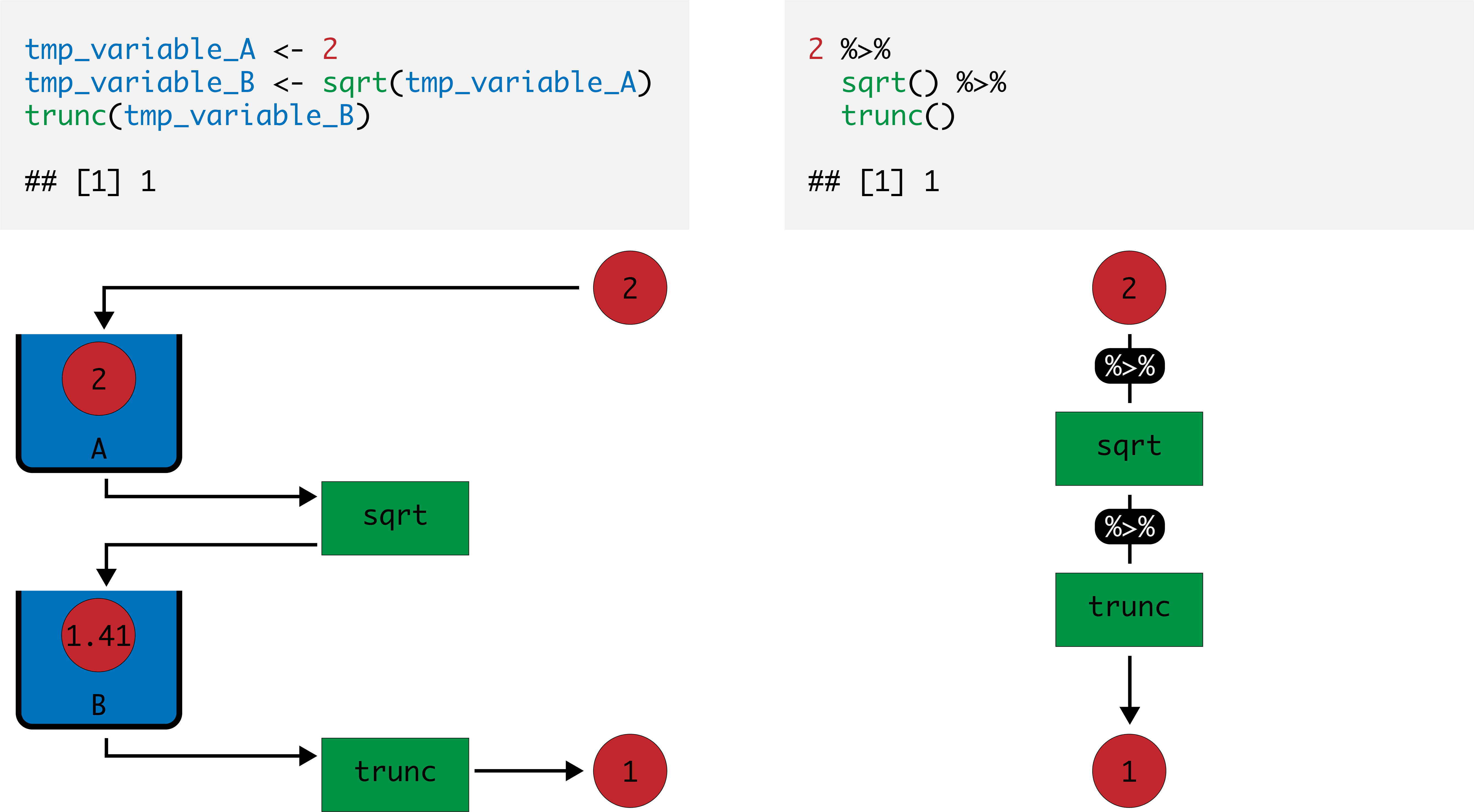
Pipe example
The two codes below are equivalent
- the first simply invokes the functions
- the second uses the pipe operator
%>%
round(sqrt(2), digits = 2)
## [1] 1.41
sqrt(2) %>%
 round(digits = 2)
## [1] 1.41
Summary
Summary
An introduction to R
- Basic types
- Basic operators
- variables
- Libraries
- The pipe operator
- Coding style
Practical session
In the practical session, we will see
- The R programming language
- Interpreting values
- Variables
- Basic types
- Tidyverse
- Coding style
Next lecture
More complex data types
- Vectors
- Factors
- Matrices
- Arrays
- Lists
- Data Frames