
2020-01-15
Recap @ 202
Previous lectures
Moving on towards data science
- Data selection
- Data filtering
- Data manipulation
This lecture
Moving on towards data science
- Join operations
- Table re-shaping
- Read and write data
Join
Joining data
Data frames can be joined (or ‘merged’)
- information from two data frames can be combined
- specifying a column with common values
- usually one with a unique identifier of an entity
- rows having the same value are joined
- depending on parameters
- a row from one data frame can be merged with multiple rows from the other data frame
- rows with no matching values in the other data frame can be retained
mergebase function or join functions indplyr
Join types
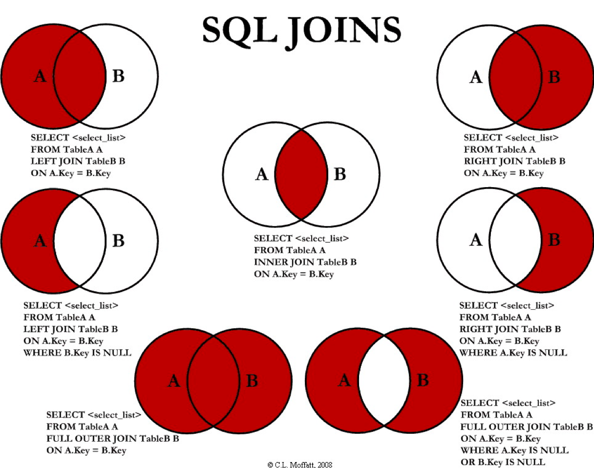
by C.L. Moffatt, licensed under The Code Project Open License (CPOL)
Example
employees <- data.frame(
  Name = c("Maria", "Pete", "Sarah", "Jo"),
  Age = c(47, 34, 32, 25),
  Role = c("Professor", "Researcher", "Researcher", "Postgrad")
)

city_of_birth <-data.frame(
  Name = c("Maria", "Pete", "Sarah", "Mel"),
  City = c("Barcelona", "London", "Boston", "Los Angeles")
)
Example
| Name | Age | Role |
|---|---|---|
| Maria | 47 | Professor |
| Pete | 34 | Researcher |
| Sarah | 32 | Researcher |
| Jo | 25 | Postgrad |
| Name | City |
|---|---|
| Maria | Barcelona |
| Pete | London |
| Sarah | Boston |
| Mel | Los Angeles |
dplyr::full_join
dplyr provides a series of join functions
full_joincombines all the available data
employees %>% full_join(
  city_of_birth,
  by = c("Name" = "Name") # join columns
  ) %>%
  kable()
| Name | Age | Role | City |
|---|---|---|---|
| Maria | 47 | Professor | Barcelona |
| Pete | 34 | Researcher | London |
| Sarah | 32 | Researcher | Boston |
| Jo | 25 | Postgrad | NA |
| Mel | NA | NA | Los Angeles |
dplyr::left_join
left_joinkeeps all the data from the left table- using
%>%, that’s the data “coming down the pipe”
- using
- rows from the right table without a match are dropped
employees %>% left_join(
  city_of_birth,
  by = c("Name" = "Name") # join columns
  ) %>%
  kable()
| Name | Age | Role | City |
|---|---|---|---|
| Maria | 47 | Professor | Barcelona |
| Pete | 34 | Researcher | London |
| Sarah | 32 | Researcher | Boston |
| Jo | 25 | Postgrad | NA |
dplyr::right_join
right_joinkeeps all the data from the right table- using
%>%, that’s the data provided as an argument
- using
- rows from the left table without a match are dropped
employees %>% right_join(
  city_of_birth,
  by = c("Name" = "Name") # join columns
  ) %>%
  kable()
| Name | Age | Role | City |
|---|---|---|---|
| Maria | 47 | Professor | Barcelona |
| Pete | 34 | Researcher | London |
| Sarah | 32 | Researcher | Boston |
| Mel | NA | NA | Los Angeles |
dplyr::inner_join
inner_joinkeeps only rows that have a match in both tables- rows without a match are dropped
employees %>% inner_join(
  city_of_birth,
  by = c("Name" = "Name") # join columns
  ) %>%
  kable()
| Name | Age | Role | City |
|---|---|---|---|
| Maria | 47 | Professor | Barcelona |
| Pete | 34 | Researcher | London |
| Sarah | 32 | Researcher | Boston |
Re-shape
Wide data
This is the most common approach
- each real-world entity is represented by one single row
- its attributes are represented through different columns
| City | Population | Area | Density |
|---|---|---|---|
| Leicester | 329,839 | 73.3 | 4,500 |
| Nottingham | 321,500 | 74.6 | 4,412 |
Long data
This is probably a less common approach, but still necessary in many cases
- each real-world entity is represented by multiple rows
- each one reporting only one of its attributes
- one column indicates which attribute each row represent
- another column is used to report the value
| City | Attribute | Value |
|---|---|---|
| Leicester | Population | 329,839 |
| Leicester | Area | 73.3 |
| Leicester | Density | 4,500 |
| Nottingham | Population | 321,500 |
| Nottingham | Area | 74.6 |
| Nottingham | Density | 4,412 |
tidyr
The tidyr (pronounced tidy-er) library is part of tidyverse and it provides functions to re-shape your data
city_info_wide <- data.frame(
  City = c("Leicester", "Nottingham"),
  Population = c(329839, 321500),
  Area = c(73.3, 74.6),
  Density = c(4500, 4412)
)

kable(city_info_wide)
| City | Population | Area | Density |
|---|---|---|---|
| Leicester | 329839 | 73.3 | 4500 |
| Nottingham | 321500 | 74.6 | 4412 |
tidyr::gather
Re-shape from wide to long format
city_info_long <- city_info_wide %>%
  gather(
    -City, # exclude city names from gathering
    key = "Attribute", # name for the new key column
    value = "Value" # name for the new value column
  )
| City | Attribute | Value |
|---|---|---|
| Leicester | Population | 329839.0 |
| Nottingham | Population | 321500.0 |
| Leicester | Area | 73.3 |
| Nottingham | Area | 74.6 |
| Leicester | Density | 4500.0 |
| Nottingham | Density | 4412.0 |
tidyr::spread
Rre-shape from long to wide format
city_info_back_to_wide <- city_info_long %>%
  spread(
    key = "Attribute", # specify key column
    value = "Value" # specify value column
  )
| City | Area | Density | Population |
|---|---|---|---|
| Leicester | 73.3 | 4500 | 329839 |
| Nottingham | 74.6 | 4412 | 321500 |
Read and write
Comma Separated Values
The file 2011_OAC_Raw_uVariables_Leicester.csv - contains data used for the 2011 Output Area Classificagtion - 167 variables, as well as the resulting groups - for the city of Leicester
Extract showing only some columns
OA11CD,LSOA11CD, ... supgrpcode,supgrpname,Total_Population, ...
E00069517,E01013785, ... 6,Suburbanites,313, ...
E00169516,E01013713, ... 4,Multicultural Metropolitans,341, ...
E00169048,E01032862, ... 4,Multicultural Metropolitans,345, ...
The full variable names can be found in the file - 2011_OAC_Raw_uVariables_Lookup.csv.
Read
The read_csv function of the readr library reads a csv file from the path provided as the first argument
leicester_2011OAC <- read_csv("2011_OAC_Raw_uVariables_Leicester.csv")

leicester_2011OAC %>%
  select(OA11CD,LSOA11CD, supgrpcode,supgrpname,Total_Population) %>%
  top_n(3) %>%
  kable()
| OA11CD | LSOA11CD | supgrpcode | supgrpname | Total_Population |
|---|---|---|---|---|
| E00169553 | E01013648 | 2 | Cosmopolitans | 714 |
| E00069303 | E01013739 | 4 | Multicultural Metropolitans | 623 |
| E00168096 | E01013689 | 2 | Cosmopolitans | 708 |
Write
The function write_csv can be used to save a dataset to csv
Example:
- read the 2011 OAC dataset
- select a few columns
- filter only those OA in the supergroup Suburbanites (code
6) - write the results to a file named Leicester_Suburbanites.csv in your home folder
read_csv("2011_OAC_Raw_uVariables_Leicester.csv") %>%
  select(OA11CD, supgrpcode, supgrpname) %>%
  filter(supgrpcode == 6) %>%
  write_csv("~/Leicester_Suburbanites.csv")
Summary
Summary
Moving on towards data science
- Join operations
- Table re-shaping
- Read and write data
Practical session
In the practical session, we will see
- Re-shaping: long and wide formats
- Join operations
- Read and write data
Next lecture
Reproducibility in (geographic) data science
- What is reproducible data analysis?
- why is it important?
- software engineering
- practical principles
- Tools
- Markdown
knitrandrmarkdown- Git