• Introduction to R
• Data types
• Data wrangling
• Reproducibility
• Exploratory analysis
  • Data visualisation
  • Descriptive statistics
  • Exploring assumptions

• Comparing means
  • t-test
  • ANOVA
• Correlation
  • Pearson’s r
  • Spearman’s rho
  • Kendall’s tau
• Regression
  • univariate

Independent T-test tests whether two group means are different

\[outcome_i = (group\ mean) + error_i \]

• groups defined by a predictor, categorical variable
• outcome is a continuous variable
• assuming
  • normally distributed values in groups
  • homogeneity of variance of values in groups
    • if groups have different sizes
  • independence of groups

Values are normally distributed, groups have same size, and they are independent (different flowers, check using leveneTest)

iris %>%
  filter(Species %in% c("versicolor", "virginica")) %$% # Note %$%
  t.test(Petal.Length ~ Species)

## 
##  Welch Two Sample t-test
## 
## data:  Petal.Length by Species
## t = -12.604, df = 95.57, p-value < 2.2e-16
## alternative hypothesis: true difference in means is not equal to 0
## 95 percent confidence interval:
##  -1.49549 -1.08851
## sample estimates:
## mean in group versicolor  mean in group virginica 
##                    4.260                    5.552

The difference is significant t(95.57) = -12.6, p < .01

ANOVA (analysis of variance) tests whether more than two group means are different

\[outcome_i = (group\ mean) + error_i \]

• groups defined by a predictor, categorical variable
• outcome is a continuous variable
• assuming
  • normally distributed values in groups
    • especially if groups have different sizes
  • homogeneity of variance of values in groups
    • if groups have different sizes
  • independence of groups

Values are normally distributed, groups have same size, they are independent (different flowers, check using leveneTest)

iris %$%
  aov(Petal.Length ~ Species) %>%
  summary()

##              Df Sum Sq Mean Sq F value Pr(>F)    
## Species       2  437.1  218.55    1180 <2e-16 ***
## Residuals   147   27.2    0.19                   
## ---
## Signif. codes:  0 '***' 0.001 '**' 0.01 '*' 0.05 '.' 0.1 ' ' 1

The difference is significant t(2, 147) = 1180.16, p < .01

Two variables can be related in three different ways

• related
  • positively: entities with high values in one tend to have high values in the other
  • negatively: entities with high values in one tend to have low values in the other
• not related at all

Correlation is a standardised measure of covariance

flights_nov_20 <- nycflights13::flights %>%
  filter(!is.na(dep_delay), !is.na(arr_delay), month == 11, day ==20) 

Combines in one visualisation: histograms, scatter plots, and correlation values for a set of variables

library(psych)

flights_nov_20 %>%
  select(
    dep_delay, 
    arr_delay, 
    air_time
  ) %>%
  pairs.panels(
    method = "kendall"
  )

Regression analysis is a supervised machine learning approach

Predict the value of one outcome variable as

\[outcome_i = (model) + error_i \]

• one predictor variable (simple / univariate regression)

\[Y_i = (b_0 + b_1 * X_{i1}) + \epsilon_i \]

• more predictor variables (multiple / multivariate regression)

\[Y_i = (b_0 + b_1 * X_{i1} + b_2 * X_{i2} + \dots + b_M * X_{iM}) + \epsilon_i \]

Least squares is the most commonly used approach to generate a regression model

The model fits a line

• to minimise the squared values of the residuals (errors)
• that is squared difference between
  • observed values
  • model

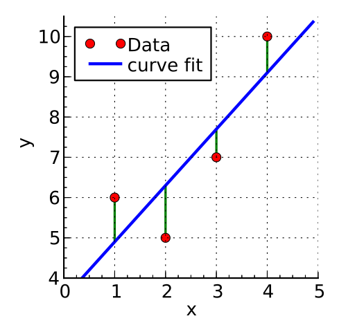
by Krishnavedala
via Wikimedia Commons,
CC-BY-SA-3.0

\[deviation = \sum(observed - model)^2\]

\[arr\_delay_i = (b_0 + b_1 * dep\_delay_{i1}) + \epsilon_i \]

delay_model <- flights_nov_20 %$% # Note %$%
  lm(arr_delay ~ dep_delay)

delay_model %>%  summary()

## 
## Call:
## lm(formula = arr_delay ~ dep_delay)
## 
## Residuals:
##     Min      1Q  Median      3Q     Max 
## -43.906  -9.022  -1.758   8.678  57.052 
## 
## Coefficients:
##             Estimate Std. Error t value Pr(>|t|)    
## (Intercept) -4.96717    0.43748  -11.35   <2e-16 ***
## dep_delay    1.04229    0.01788   58.28   <2e-16 ***
## ---
## Signif. codes:  0 '***' 0.001 '**' 0.01 '*' 0.05 '.' 0.1 ' ' 1
## 
## Residual standard error: 13.62 on 972 degrees of freedom
## Multiple R-squared:  0.7775, Adjusted R-squared:  0.7773 
## F-statistic:  3397 on 1 and 972 DF,  p-value: < 2.2e-16

The output indicates

• p-value: < 2.2e-16: \(p<.001\) the model is significant
  • derived by comparing the calulated F-statistic value to F distribution 3396.74 having specified degrees of freedom (1, 972)
  • Report as: F(1, 972) = 3396.74
• Adjusted R-squared: 0.7773: the departure delay can account for 77.73% of the arrival delay
• Coefficients
  • Intercept estimate -4.9672 is significant
  • dep_delay (slope) estimate 1.0423 is significant

\[arr\_delay_i = (Intercept + Coefficient_{dep\_delay} * dep\_delay_{i1}) + \epsilon_i \]

flights_nov_20 %>%
  ggplot(aes(x = dep_delay, y = arr_delay)) +
  geom_point() + coord_fixed(ratio = 1) +
  geom_abline(intercept = 4.0943, slope = 1.04229, color="red")

• Linearity
  • the relationship is actually linear
• Normality of residuals
  • standard residuals are normally distributed with mean 0
• Homoscedasticity of residuals
  • at each level of the predictor variable(s) the variance of the standard residuals should be the same (homo-scedasticity) rather than different (hetero-scedasticity)
• Independence of residuals
  • adjacent standard residuals are not correlated
• When more than one predictor: no multicollinearity
  • if two or more predictor variables are used in the model, each pair of variables not correlated

Shapiro-Wilk test for normality of standard residuals,

• robust models: should be not significant

delay_model %>% 
  rstandard() %>% 
  shapiro.test()

## 
##  Shapiro-Wilk normality test
## 
## data:  .
## W = 0.98231, p-value = 1.73e-09

Standard residuals are NOT normally distributed

Breusch-Pagan test for homoscedasticity of standard residuals

• robust models: should be not significant

library(lmtest)

delay_model %>% 
  bptest()

## 
##  studentized Breusch-Pagan test
## 
## data:  .
## BP = 0.017316, df = 1, p-value = 0.8953

Durbin-Watson test for the independence of residuals

• robust models: statistic should be close to 2 (between 1 and 3) and not significant

# Also part of the library lmtest
delay_model %>%
  dwtest()

## 
##  Durbin-Watson test
## 
## data:  .
## DW = 1.8731, p-value = 0.02358
## alternative hypothesis: true autocorrelation is greater than 0

Standard residuals might not be completely indipendent

Note: the result depends on the order of the data.

• Comparing means
  • t-test
  • ANOVA
• Correlation
  • Pearson’s r
  • Spearman’s rho
  • Kendall’s tau
• Regression
  • univariate

In the practical session, we will see:

• Comparing means
  • ANOVA
• Regression
  • univariate
  • multivariate

• Machine Learning
  • Definition
  • Types
• Unsupervised
  • Clustering
• In GIScience
  • Geodemographic classification