
2020-01-15
Recap @ 601
Previous lectures
- Introduction to R
- Data types
- Data wrangling
- Reproducibility
- Exploratory analysis
- Univariate analysis
- Correlation
- Regression
This lecture
- Machine Learning
- Definition
- Types
- Unsupervised
- Clustering
- In GIScience
- Geodemographic classification
Lecture 601
Machine Learning
Definition
“The field of machine learning is concerned with the question of how to construct computer programs that automatically improve with experience.”
Mitchell, T. (1997). Machine Learning. McGraw Hill.
Origines
- Computer Science:
- how to manually program computers to solve tasks
- Statistics:
- what conclusions can be inferred from data
- Machine Learning:
- intersection of computer science and statistics
- how to get computers to program themselves from experience plus some initial structure
- effective data capture, store, index, retrieve and merge
- computational tractability
Mitchell, T.M., 2006. The discipline of machine learning (Vol. 9). Pittsburgh, PA: Carnegie Mellon University, School of Computer Science, Machine Learning Department.
Types of machine learning
Machine learning approaches are divided into two main types
- Supervised
- training of a “predictive” model from data
- one attribute of the dataset is used to “predict” another attribute
- e.g., classification
- Unsupervised
- discovery of descriptive patterns in data
- commonly used in data mining
- e.g., clustering
Supervised
- Training dataset
- input attribute(s)
- attribute to predict
- Testing dataset
- input attribute(s)
- attribute to predict
- Type of learning model
- Evaluation function
- evaluates difference between prediction and output in testing data
by Josef Steppan
via Wikimedia Commons,
CC-BY-SA-4.0
Unsupervised
- Dataset
- input attribute(s) to explore
- Type of model for the learning process
- most approaches are iterative
- e.g., hierarchical clustering
- Evaluation function
- evaluates the quality of the pattern under consideration during one iteration
by Chire
via Wikimedia Commons,
CC-BY-SA-3.0
… more
- Semi-supervised learning
- between unsupervised and supervised learning
- combines a small amount of labelled data with a larger un-labelled dataset
- continuity, cluster, and manifold (lower dimensionality) assumption
- Reinforcement learning
- training agents take actions to maximize reward
- balancing
- exploration (new paths/options)
- exploitation (of current knowledge)
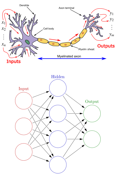
Neural networks
Supervised learning approach simulating simplistic neurons
- Classic model with 3 sets
- input neurons
- output neurons
- hidden layer
- combines input values using weights
- activation function
- The traning algorithm is used to define the best weights
by Egm4313.s12 and Glosser.ca
via Wikimedia Commons,
CC-BY-SA-3.0
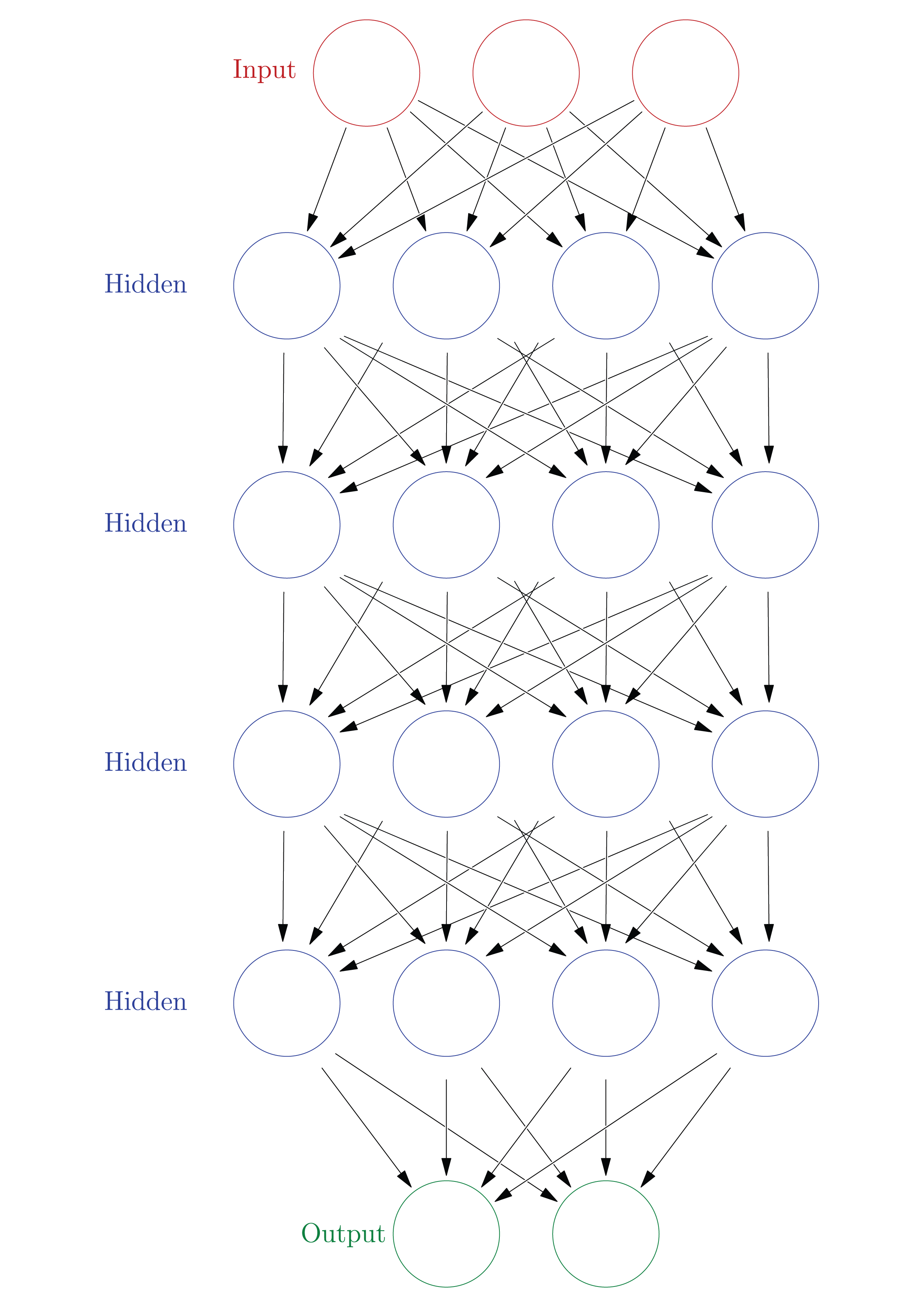
Deep neural networks
Neural networks with multiple hidden layers
The fundamental idea is that “deeper” neurons allow for the encoding of more complex characteristics
Example: De Sabbata, S. and Liu, P. (2019). Deep learning geodemographics with autoencoders and geographic convolution. In proceedings of the 22nd AGILE Conference on Geographic Information Science, Limassol, Cyprus.
derived from work by Glosser.ca
via Wikimedia Commons,
CC-BY-SA-3.0
Convolutional neural networks
Deep neural networks with convolutional hidden layers
- used very successfully on image object recognition
- convolutional hidden layers “convolve” the images
- a process similar to applying smoothing filters
Example: Liu, P. and De Sabbata, S. (2019). Learning Digital Geographies through a Graph-Based Semi-supervised Approach. In proceedings of the 15th International Conference on GeoComputation, Queenstown, New Zealand.
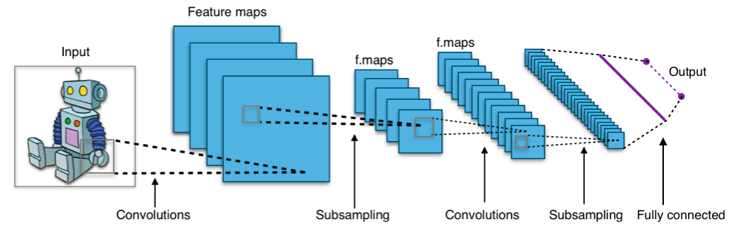
by Aphex34 via Wikimedia Commons, CC-BY-SA-4.0
Limits
- Complexity
- Training dataset quality
- garbage in, garbage out
- e.g., Facial Recognition Is Accurate, if You’re a White Guy by Steve Lohr (New York Times, Feb. 9, 2018)
- Overfitting
- creating a model perfect for the training data, but not generic enough to be useful
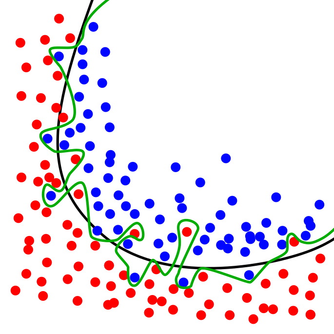
by Chabacano
ia Wikimedia Commons,
CC-BY-SA-4.0
Lecture 601
Clustering
Clustering task
"Clustering is an unsupervised machine learning task that automatically divides the data into clusters , or groups of similar items". (Lantz, 2019)
Methods:
- Centroid-based
- k-means
- fuzzy c-means
- Hierarchical
- Mixed
- bootstrap aggregating
- Density-based
- DBSCAN
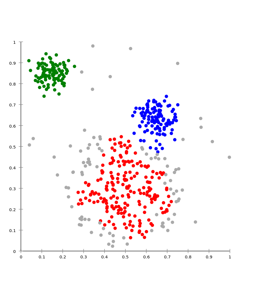
Example
data_to_cluster <- data.frame(
  x_values = c(rnorm(40, 5, 1), rnorm(60, 10, 1), rnorm(20, 12, 3)),
  y_values = c(rnorm(40, 5, 1), rnorm(60, 5, 3), rnorm(20, 15, 1)),
  original_group = c(rep("A", 40), rep("B", 60), rep("C", 20)) )

k-means
k-mean clusters n observations in k clusters, minimising the within-cluster sum of squares (WCSS)
Algorithm: k observations a randomly selected as initial centroids, then repeat
- assignment step: observations are assigned to the closest centroids
- update step: calculate means for each cluster to use as new the centroid
until centroids don’t change anymore, the algorithm has converged
kmeans_found_clusters <- data_to_cluster %>%
  select(x_values, y_values) %>%
  kmeans(centers=3, iter.max=50)

data_to_cluster <- data_to_cluster %>%
  add_column(kmeans_cluster = kmeans_found_clusters$cluster)
K-means result

Fuzzy c-means
Fuzzy c-means is similar to k-means but allows for "fuzzy" membership to clusters
Each observation is assigned with a value per each cluster
- usually from
0to1 - indicates how well the observation fits within the cluster
- i.e., based on the distance from the centroid
library(e1071)

cmeans_result <- data_to_cluster %>%
  select(x_values, y_values) %>%
  cmeans(centers=3, iter.max=50)

data_to_cluster <- data_to_cluster %>%
  add_column(c_means_assigned_cluster = cmeans_result$cluster)
Fuzzy c-means
A “crisp” classification can be created by picking the highest membership value.
- that also allows to set a membership threshold (e.g.,
0.75) - leaving some observations without a cluster
data_to_cluster <- data_to_cluster %>%
  add_column(
    c_means_membership = apply(cmeans_result$membership, 1, max)
  ) %>%
  mutate(
    c_means_cluster = ifelse(
      c_means_membership > 0.75,
      c_means_assigned_cluster,
      0
    )
  )
Fuzzy c-means result

Hierarchical clustering
Algorithm: each object is initialised as, then repeat
- join the two most similar clusters based on a distance-based metric
- e.g., Ward’s (1963) approach is based on variance
until only one single cluster is achieved
hclust_result <- data_to_cluster %>%
  select(x_values, y_values) %>%
  dist(method="euclidean") %>%
  hclust(method="ward.D2")

data_to_cluster <- data_to_cluster %>%
  add_column(hclust_cluster = cutree(hclust_result, k=3))
Clustering tree
This approach generates a clustering tree (dendrogram), which can then be “cut” at the desired height
plot(hclust_result) + abline(h = 30, col = "red")

## integer(0)
Hierarchical clustering result

Bagged clustering
Bootstrap aggregating (b-agg-ed) clustering approach (Leisch, 1999)
- first k-means on samples
- then a hierarchical clustering of the centroids generated through the samples
library(e1071)

bclust_result <- data_to_cluster %>%
  select(x_values, y_values) %>%
  bclust(hclust.method="ward.D2", resample = TRUE)

data_to_cluster <- data_to_cluster %>%
  add_column(bclust_cluster = clusters.bclust(bclust_result, 3))
Bagged clustering result

Density based clustering
DBSCAN (“density-based spatial clustering of applications with noise”) starts from an unclustered point and proceeds by aggregating its neighbours to the same cluster, as long as they are within a certain distance. (Ester et al, 1996)
library(dbscan)

dbscan_result <- data_to_cluster %>%
  select(x_values, y_values) %>%
   dbscan(eps = 1, minPts = 5)

data_to_cluster <- data_to_cluster %>%
  add_column(dbscan_cluster = dbscan_result$cluster)
DBSCAN result

Geodemographic classifications
In GIScience, the clustering is commonly used to create geodemographic classifications such as the 2011 Output Area Classification (Gale et al., 2016)
- initial set of 167 prospective variables from the United Kingdom Census 2011
- 86 were removed,
- 41 were retained as they are
- 40 were combined
- final set of 60 variables.
- k-means clustering approach to create
- 8 supergroups
- 26 groups
- 76 subgroups.
Lecture 601
Summary
Summary
- Machine Learning
- Definition
- Types
- Unsupervised
- Clustering
- In GIScience
- Geodemographic classification
Practical session
In the practical session we will see:
Geodemographic classification in R