5 Data wrangling Pt. 2

Stefano De Sabbata

This work is licensed under the GNU General Public License v3.0. Contains public sector information licensed under the Open Government Licence v3.0.

This section illustrates the re-shape and join functionalities of the Tidyverse libraries using simple examples. The following sections instead present a more complex example, loading and wrangling with data related to the 2011 Output Area Classification and the Indexes of Multiple Deprivation 2015.

library(tidyverse)
library(knitr)

5.1 Table manipulation

5.1.1 Long and wide formats

Tabular data are usually presented in two different formats.

Wide: this is the most common approach, where each real-world entity (e.g. a city) is represented by one single row and its attributes are represented through different columns (e.g., a column representing the total population in the area, another column representing the size of the area, etc.).

City	Population	Area	Density
Leicester	329,839	73.3	4,500
Nottingham	321,500	74.6	4,412

Long: this is probably a less common approach, but still necessary in many cases, where each real-world entity (e.g. a city) is represented by multiple rows, each one reporting only one of its attributes. In this case, one column is used to indicate which attribute each row represent, and another column is used to report the value.

City	Attribute	Value
Leicester	Population	329,839
Leicester	Area	73.3
Leicester	Density	4,500
Nottingham	Population	321,500
Nottingham	Area	74.6
Nottingham	Density	4,412

The tidyr library provides two functions that allow transforming wide-formatted data to a long format, and vice-versa. Please take your time to understand the example below and check out the tidyr help pages before continuing.

city_info_wide <- data.frame(
  City = c("Leicester", "Nottingham"),
  Population = c(329839, 321500),
  Area = c(73.3, 74.6),
  Density = c(4500, 4412)
)

kable(city_info_wide)

City	Population	Area	Density
Leicester	329839	73.3	4500
Nottingham	321500	74.6	4412

city_info_long <- city_info_wide %>%
  gather(
    # exclude IDs (city names) from gathering
    -City,
    # name for the new key column
    key = "Attribute",
    # name for the new value column
    value = "Value"
  )

kable(city_info_long)

City	Attribute	Value
Leicester	Population	329839.0
Nottingham	Population	321500.0
Leicester	Area	73.3
Nottingham	Area	74.6
Leicester	Density	4500.0
Nottingham	Density	4412.0

city_info_back_to_wide <- city_info_long %>%
  spread(
    # specify key column
    key = "Attribute",
    # specify value column
    value = "Value"
  )

kable(city_info_back_to_wide)

City	Area	Density	Population
Leicester	73.3	4500	329839
Nottingham	74.6	4412	321500

5.1.2 Join

A join operation combines two tables into one by matching rows that have the same values in the specified column. This operation is usually executed on columns containing identifiers, which are matched through different tables containing different data about the same real-world entities. For instance, the table below presents the telephone prefixes for two cities. That information can be combined with the data present in the wide-formatted table above through a join operation on the columns containing the city names. As the two tables do not contain all the same cities, if a full join operation is executed, some cells have no values assigned.

City	TelephonePrefix
Leicester	0116
Birmingham	0121

City	Population	Area	Density	TelephonePrefix
Leicester	329,839	73.3	4,500	0116
Nottingham	321,500	74.6	4,412
Birmingham				0121

As discussed in the lecture, the dplyr library offers different types of join operations, which correspond to the different SQL joins illustrated in the image below. The use and implications of these different types of joins will be discussed in more detail in the GY7708 module next semester.

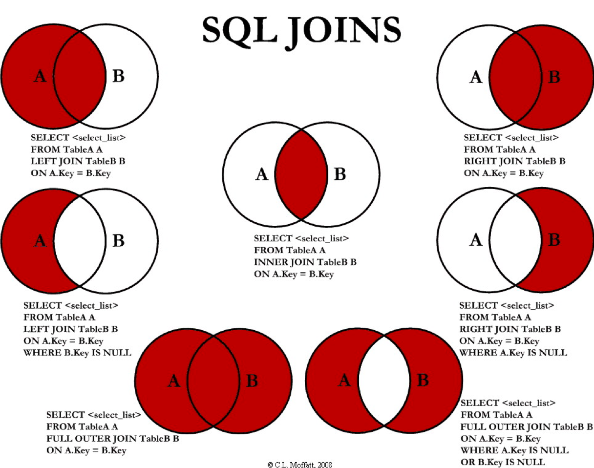
by C.L. Moffatt, licensed under The Code Project Open License (CPOL)

Please take your time to understand the example below and check out the related dplyr help pages before continuing. Note how the result of the join operations is not saved to a variable. The function kable is added after each join operation through a pipe %>% to display the resulting table in a nice format.

city_telephone_prexix <- data.frame(
  City = c("Leicester", "Birmingham"),
  TelephonPrefix = c("0116", "0121")
)

kable(city_telephone_prexix)

City	TelephonPrefix
Leicester	0116
Birmingham	0121

full_join(
    city_info_wide, city_telephone_prexix,
    by = c("City" = "City")
  ) %>%
  kable()

City	Population	Area	Density	TelephonPrefix
Leicester	329839	73.3	4500	0116
Nottingham	321500	74.6	4412	NA
Birmingham	NA	NA	NA	0121

left_join(
    city_info_wide, city_telephone_prexix,
    by = c("City" = "City")
  ) %>%
  kable()

City	Population	Area	Density	TelephonPrefix
Leicester	329839	73.3	4500	0116
Nottingham	321500	74.6	4412	NA

right_join(
    city_info_wide, city_telephone_prexix,
    by = c("City" = "City")
  ) %>%
  kable()

City	Population	Area	Density	TelephonPrefix
Leicester	329839	73.3	4500	0116
Birmingham	NA	NA	NA	0121

inner_join(
    city_info_wide, city_telephone_prexix,
    by = c("City" = "City")
  ) %>%
  kable()

City	Population	Area	Density	TelephonPrefix
Leicester	329839	73.3	4500	0116

5.2 Read and write data

The readr library (also part of the Tidyverse) provides a series of functions that can be used to load from and save data to different file formats.

Download from the Data folder of the repository the following files:

2011_OAC_Raw_uVariables_Leicester.csv
IndexesMultipleDeprivation2015_Leicester.csv

Create a Practical_202 project and make sure it is activated and thus the Practical_202 showing in the File tab in the bottom-right panel. Upload the two files to the Practical_202 folder by clicking on the Upload button and selecting the files from your computer (at the time of writing, Chrome seems to upload the file correctly, whereas it might be necessary to change the names of the files after upload using Microsoft Edge).

Create a new R script named Data_Wrangling_Example.R in the Practical_202 project, and add library(tidyverse) as the first line. Use that new script for this and the following sections of this practical session.

The 2011 Output Area Classification (2011 OAC) is a geodemographic classification of the census Output Areas (OA) of the UK, which was created by Gale et al. (2016) starting from an initial set of 167 prospective variables from the United Kingdom Census 2011: 86 were removed, 41 were retained as they are, and 40 were combined, leading to a final set of 60 variables. Gale et al. (2016) finally used the k-means clustering approach to create 8 clusters or supergroups (see map at datashine.org.uk), as well as 26 groups and 76 subgroups. The dataset in the file 2011_OAC_Raw_uVariables_Leicester.csv contains all the original 167 variables, as well as the resulting groups, for the city of Leicester. The full variable names can be found in the file 2011_OAC_Raw_uVariables_Lookup.csv.

The Indexes of Multiple Deprivation 2015 (see map at cdrc.ac.uk) are based on a series of variables across seven distinct domains of deprivation which are combined to calculate the Index of Multiple Deprivation 2015 (IMD 2015). That is an overall measure of multiple deprivations experienced by people living in an area. These indexes are calculated for every Lower layer Super Output Area (LSOA), which are larger geographic unit than the OAs used for the 2011 OAC. The dataset in the file IndexesMultipleDeprivation2015_Leicester.csv contains the main Index of Multiple Deprivation, as well as the values for the seven distinct domains of deprivation, and two additional indexes regarding deprivation affecting children and older people. The dataset includes scores, ranks (where 1 indicates the most deprived area), and decile (i.e., the first decile includes the 10% most deprived areas in England).

The read_csv function reads a Comma Separated Values (CSV) file from the path provided as the first argument. The code below loads the 2011 OAC dataset. The read_csv instruction throws a warning that shows the assumptions about the data types used when loading the data. As illustrated by the output of the last line of code, the data are loaded as a tibble 969 x 190, that is 969 rows – one for each OA – and 190 columns, 167 of which represent the input variables used to create the 2011 OAC.

leicester_2011OAC <- read_csv("2011_OAC_Raw_uVariables_Leicester.csv")

leicester_2011OAC %>% 
  select(OA11CD,LSOA11CD, supgrpcode,supgrpname,Total_Population) %>%
  top_n(3) %>%
  kable()

OA11CD	LSOA11CD	supgrpcode	supgrpname	Total_Population
E00169553	E01013648	2	Cosmopolitans	714
E00069303	E01013739	4	Multicultural Metropolitans	623
E00168096	E01013689	2	Cosmopolitans	708

The code below loads the IMD 2015 dataset.

# Load Indexes of Multiple deprivation data
leicester_IMD2015 <- read_csv("IndexesMultipleDeprivation2015_Leicester.csv")

The function write_csv can be used to save a dataset as a csv file. For instance, the code below uses tidyverse functions and the pipe operator %>% to:

read the 2011 OAC dataset again directly from the file, but without storing it into a variable;
select the OA code variable OA11CD, and the two variables representing the code and name of the supergroup assigned to each OA by the 2011 OAC (supgrpcode and supgrpname respectively);
filter only those OA in the supergroup Suburbanites (code 6);
write the results to a file named Leicester_Suburbanites.csv in your home folder.

read_csv("2011_OAC_Raw_uVariables_Leicester.csv") %>%
  select(OA11CD, supgrpcode, supgrpname) %>%
  filter(supgrpcode == 6) %>%
  write_csv("~/Leicester_Suburbanites.csv")

5.3 Data wrangling example

5.3.1 Re-shaping

The IMD 2015 data are in a long format, which means that every area is represented by more than one row: the column Value presents the value; the column IndicesOfDeprivation indicates which index the value refers to; the column Measurement indicates whether the value is a score, rank, or decile. The code below illustrates the data format for the LSOA including the University of Leicester (feature code E01013649).

leicester_IMD2015 %>%
  filter(FeatureCode == "E01013649") %>%
  select(FeatureCode, IndicesOfDeprivation, Measurement, Value)

## # A tibble: 30 x 4
##    FeatureCode IndicesOfDeprivation                      Measurement  Value
##    <chr>       <chr>                                     <chr>        <dbl>
##  1 E01013649   Income Deprivation Domain                 Score        0.07 
##  2 E01013649   Employment Deprivation Domain             Score        0.075
##  3 E01013649   Income Deprivation Affecting Children In… Score        0.087
##  4 E01013649   Income Deprivation Affecting Older Peopl… Score        0.153
##  5 E01013649   Health Deprivation and Disability Domain  Score        0.272
##  6 E01013649   Index of Multiple Deprivation (IMD)       Score       19.7  
##  7 E01013649   Education, Skills and Training Domain     Score        2.19 
##  8 E01013649   Barriers to Housing and Services Domain   Score       14.3  
##  9 E01013649   Living Environment Deprivation Domain     Score       57.2  
## 10 E01013649   Crime Domain                              Score        1.16 
## # … with 20 more rows

In the following section, the analysis aims to explore how certain census variables vary in areas with different deprivation levels. Thus, we need to extract the Decile rows from the IMD 2015 dataset and transform the data in a wide format, where each index is represented as a separate column.

To that purpose, we also need to change the name of the indexes slightly, to exclude spaces and punctuation, so that the new column names are simpler than the original text, and can be used as column names. That part of the manipulation is performed using mutate and functions from the stringr library.

leicester_IMD2015_decile_wide <- leicester_IMD2015 %>%
  # Select only Socres
  filter(Measurement == "Decile") %>%
  # Trim names of IndicesOfDeprivation
  mutate(IndicesOfDeprivation = str_replace_all(IndicesOfDeprivation, "\\s", "")) %>%
  mutate(IndicesOfDeprivation = str_replace_all(IndicesOfDeprivation, "[:punct:]", "")) %>%
  mutate(IndicesOfDeprivation = str_replace_all(IndicesOfDeprivation, "\\(", "")) %>%
  mutate(IndicesOfDeprivation = str_replace_all(IndicesOfDeprivation, "\\)", "")) %>%
  # Spread
  spread(
    key = IndicesOfDeprivation,
    value = Value
  ) %>%
  # Drop columns
  select(-DateCode, -Measurement, -Units)

Let’s compare the columns of the original long IMD 2015 dataset with the wide dataset created above.

colnames(leicester_IMD2015)

## [1] "FeatureCode"          "DateCode"             "Measurement"         
## [4] "Units"                "Value"                "IndicesOfDeprivation"

colnames(leicester_IMD2015_decile_wide)

##  [1] "FeatureCode"                                     
##  [2] "BarrierstoHousingandServicesDomain"              
##  [3] "CrimeDomain"                                     
##  [4] "EducationSkillsandTrainingDomain"                
##  [5] "EmploymentDeprivationDomain"                     
##  [6] "HealthDeprivationandDisabilityDomain"            
##  [7] "IncomeDeprivationAffectingChildrenIndexIDACI"    
##  [8] "IncomeDeprivationAffectingOlderPeopleIndexIDAOPI"
##  [9] "IncomeDeprivationDomain"                         
## [10] "IndexofMultipleDeprivationIMD"                   
## [11] "LivingEnvironmentDeprivationDomain"

Thus, we now have only one row representing the LSOA including the University of Leicester (feature code E01013649) and the main Index of Multiple Deprivations is now represented by the column IndexofMultipleDeprivationIMD. The value reported is the same – that is 5, which means that the selected LSOA is estimated to be in the range 40-50% most deprived areas in England – but we changed the data format.

# Original long IMD 2015 dataset
leicester_IMD2015 %>%
  filter(
    FeatureCode == "E01013649",
    IndicesOfDeprivation == "Index of Multiple Deprivation (IMD)",
    Measurement == "Decile"
  ) %>%
  select(FeatureCode, IndicesOfDeprivation, Measurement, Value)

## # A tibble: 1 x 4
##   FeatureCode IndicesOfDeprivation                Measurement Value
##   <chr>       <chr>                               <chr>       <dbl>
## 1 E01013649   Index of Multiple Deprivation (IMD) Decile          5

# New wide IMD 2015 dataset
leicester_IMD2015_decile_wide %>%
  filter(FeatureCode == "E01013649") %>%
  select(FeatureCode, IndexofMultipleDeprivationIMD)

## # A tibble: 1 x 2
##   FeatureCode IndexofMultipleDeprivationIMD
##   <chr>                               <dbl>
## 1 E01013649                               5

5.3.2 Join

As discussed above, two tables can be joined using a common column of identifiers. We can thus join the 2011 OAC and the IMD 2015 datasets into a single table. The LSOA code included in the 2011 OAC table is used to match that information with the corresponding row in the IMD 2015. The resulting table provides all the information from the 2011 OAC for each OA, plus the Index of Multiple Deprivations decile for the LSOA containing each OA.

That operation can be carried out using the function merge, and specifying the common column (or columns, if more than one is to be used as identifier) as argument of by.

leicester_2011OAC_IMD2015 <- leicester_2011OAC %>%
  left_join(leicester_IMD2015_decile_wide, by = c("LSOA11CD" = "FeatureCode"))

Once the result is stored into the variable leicester_2011OAC_IMD2015, further analysis can be carried out. For instance, count can be used to count how many OAs fall into each 2011 OAC supergroup and decile of the Index of Multiple Deprivations.

leicester_2011OAC_IMD2015 %>%
  count(supgrpname, IndexofMultipleDeprivationIMD)

## # A tibble: 46 x 3
##    supgrpname                IndexofMultipleDeprivationIMD     n
##    <chr>                                             <dbl> <int>
##  1 Constrained City Dwellers                             1    30
##  2 Constrained City Dwellers                             2     3
##  3 Constrained City Dwellers                             3     2
##  4 Constrained City Dwellers                             6     1
##  5 Cosmopolitans                                         2    25
##  6 Cosmopolitans                                         3    15
##  7 Cosmopolitans                                         4    15
##  8 Cosmopolitans                                         5     8
##  9 Cosmopolitans                                         6    10
## 10 Cosmopolitans                                         8    10
## # … with 36 more rows

As another example, the code below can be used to group OAs based on the decile and then calculate the percentage of adults not in employment using the u074 (No adults in employment in household: With dependent children) and u075 (No adults in employment in household: No dependent children) variables from the 2011 OAC dataset.

leicester_2011OAC_IMD2015 %>%
  group_by(IndexofMultipleDeprivationIMD) %>%
  summarise(
    adults_not_empl_perc = (sum(u074 + u075) / sum(Total_Population)) * 100
  ) %>%
  kable()

IndexofMultipleDeprivationIMD	adults_not_empl_perc
1	17.071876
2	14.191205
3	10.405029
4	9.966309
5	11.337036
6	10.710509
7	10.641026
8	9.686658
9	9.898140

5.4 Exercise 3.1

Extend the code in the script Data_Wrangling_Example.R to include the code necessary to solve the questions below.

Question 3.1.1: Write a piece of code using the pipe operator and the dplyr library to generate a table showing the percentage of EU citizens over total population, calculated grouping OAs by the related decile of the Index of Multiple Deprivations, but only accounting for areas classified as Cosmopolitans or Ethnicity Central or Multicultural Metropolitans.

Question 3.1.2: Write a piece of code using the pipe operator and the dplyr library to generate a table showing the percentage of EU citizens over total population, calculated grouping OAs by the related supergroup in the 2011 OAC, but only accounting for areas in the top 5 deciles of the Index of Multiple Deprivations.

Question 3.1.3: Write a piece of code using the pipe operator and the dplyr library to generate a table showing the percentage of people aged 65 and above, calculated grouping OAs by the related supergroup in the 2011 OAC and decile of the Index of Multiple Deprivations, and ordering the table by the calculated value in a descending order.

5.5 Exercise 3.2

Extend the code in the script Data_Wrangling_Example.R to include the code necessary to solve the questions below.

Question 3.2.1: Write a piece of code using the pipe operator and the dplyr and tidyr libraries to generate a long format of the leicester_2011OAC_IMD2015 table only including the values (census variables) used in Question 3.1.3.

Question 3.2.2: Write a piece of code using the pipe operator and the dplyr and tidyr libraries to generate a table similar to the one generated for Question 3.2.1, but showing the values as percentages over total population.

5.6 Solutions

A full R Script including the code for the analysis presented in this practical session and the solutions to the 5 questions above is available in the Exercise folder of the repository (202_X_Data_Wrangling2_Example.R). Upload the prepared script to your Practical_202 project folder, click on the uploaded file to open it in a new editor tab and compare it to your script.