1 Introduction to R

This work is licensed under the GNU General Public License v3.0.

1.1 The R programming language

As mentioned in Lecture 1, R was created in 1992 by Ross Ihaka and Robert Gentleman at the University of Auckland, New Zealand. R is a free, open-source implementation of the S statistical programming language initially created at the Bell Labs. At its core, R is a functional programming language (its main functionalities revolve around defining and executing functions). However it now supports, and it is commonly used as an imperative (focused on instructions on variables and programming control structures) and object-oriented (involving complex object structures) programming language.

In simple terms, nowadays, programming in R mostly focuses on devising a series of instructions to execute a task – most commonly, loading and analysing a dataset.

As such, R can be used to program creating sequences of instructions involving variables – which are named entities that can store values. That will be the main topic of the first and second weeks. Instructions can include control flow structures, such as decision points (if/else) and loops, which will be the topic of the third lecture and practical session. Instructions can also be grouped in functions, which we will see in the fourth lecture and practical session.

R is interpreted, not compiled. Which means that an R interpreter (if you are using R Studio, the R interpreter is simply hidden in the backend and R Studio is the frontend that allows you to interact with the interpreter) receives an instruction you write in R, interprets and executes them. Other programming languages require their code to be compiled in an executable in order to be executed on a computer.

1.1.1 Using RStudio

As you open RStudio or RStudio Server, the interface is divided into two main sections. On the left side, you find the Console – as well as the R script editor, when a script is being edited. The Console in an input/output window into the R interpreter, where instructions can be typed, and the computed output is shown.

For instance, if you type in the Console

1 + 1

the R interpreter understands that as an instruction to sum one to one, and produces the result (as the materials for this module are created in RMarkdown, the output of computation is always preceded by ‘##’).

## [1] 2

Note how the output value 2 is preceded by [1], which indicates that the output is constituted by only one element. If the output is constituted by more than one element, as the list of numbers below, each row of the output is preceded by the index of the first element of the output.

##  [1]   1   4   9  16  25  36  49  64  81 100 121 144 169 196 225 256 289
## [18] 324 361 400

On the right side, you find two groups of panels. On the top-right, the main element is the Environment panel, which is a representation of the current state of the interpreter’s memory, and as such, it shows all the stored variables, datasets, and functions. On the bottom-right, you find the Files panel, which shows file system (file and folders on your computer or the server), as well as the Help panel, which shows you the help pages when required. We will discuss the other panels later on in the practical sessions.

1.2 Interpreting values

When a value is typed in the Console, the interpreter simply returns the same value. In the examples below, 2 is a simple numeric value, while "String value" is a textual value, which in R is referred to as a character value and in programming is also commonly referred to as a string (short for a string of characters).

Numeric example:

## [1] 2

Character example:

"String value"

## [1] "String value"

Note how character values need to start and end with a single or double quote (' or "), which are not part of the information themselves. The Tidyverse Style Guide suggests always to use the double quote ("), so we will use those in this module.

Anything that follows a # symbol is considered a comment and the interpreter ignores it.

# hi, I am a comment, please ignore me

As mentioned above, the interpreter understands simple operations on numeric values.

1 + 1

## [1] 2

There are also a large number of pre-defined functions, e.g., square-root: sqrt.

sqrt(2)

## [1] 1.414214

Functions are collected and stored in libraries (sometimes referred to as packages), which contains related functions. Libraries can range anywhere from the base library, which includes the sqrt function above, to the rgdal library, which contains implementations of the GDAL (Geospatial Data Abstraction Library) functionalities for R.

1.3 Variables

A variable can be defined using an identifier (e.g., a_variable) on the left of an assignment operator <-, followed by the object to be linked to the identifier, such as a value (e.g., 1) to be assigned on the right. The value of the variable can be tested/invoked by simply specifying the identifier.

a_variable <- 1
a_variable

## [1] 1

If you type a_variable <- 1 in the Console in RStudio, a new element appears in the Environment panel, representing the new variable in the memory. The left part of the entry contains the identifier a_variable, and the right part contains the value assigned to the variable a_variable, that is 1.

It is not necessary to provide a value directly. The right part of the assignment can be a call to a function. In that case, the function is executed on the provided input and the result is assigned to the variable.

a_variable <- sqrt(4)
a_variable

## [1] 2

Note how if you type a_variable <- sqrt(4) in the Console in RStudio, the element in the Environment panel changes to reflect the new value assigned to the variable a_variable, which is now the result of sqrt(4), that is 2.

In the example below, another variable named another_variable is created and summed to a_variable, saving the result in sum_of_two_variables. The square root of that sum is then stored in the variable square_root_of_sum.

another_variable <- 4
another_variable

## [1] 4

sum_of_two_variables <- a_variable + another_variable

square_root_of_sum <- sqrt(sum_of_two_variables)
square_root_of_sum

## [1] 2.44949

1.4 Basic types

1.4.1 Numeric

The numeric type represents numbers (both integers and reals).

a_number <- 1.41
is.numeric(a_number)

## [1] TRUE

is.integer(a_number)

## [1] FALSE

is.double(a_number) # i.e., is real

## [1] TRUE

Base numeric operators.

Operator	Meaning	Example	Output
+	Plus	`5+2`	7
-	Minus	`5-2`	3
`*`	Product	`5*2`	10
/	Division	`5/2`	2.5
%/%	Integer division	`5%/%2`	2
%%	Module	`5%%2`	1
^	Power	`5^2`	25

Some pre-defined functions in R:

abs(-2) # Absolute value

## [1] 2

ceiling(3.475) # Upper round

## [1] 4

floor(3.475) # Lower round

## [1] 3

trunc(5.99) # Truncate

## [1] 5

log10(100) # Logarithm 10

## [1] 2

log(exp(2)) # Natural logarithm and e

## [1] 2

Use simple brackets to specify the order of execution. If not specified the default order is: rise to power first, then multiplication and division, sum and subtraction last.

a_number <- 1
(a_number + 2) * 3

## [1] 9

a_number + (2 * 3)

## [1] 7

a_number + 2 * 3

## [1] 7

The object NaN (Not a Number) is returned by R when the result of an operation is not a number.

0 / 0

## [1] NaN

is.nan(0 / 0)

## [1] TRUE

That is not to be confused with the object NA (Not Available), which is returned for missing data.

1.4.2 Logical

The logical type encodes two truth values: True and False.

logical_var <- TRUE
is.logical(logical_var)

## [1] TRUE

isTRUE(logical_var)

## [1] TRUE

as.logical(0) # TRUE if not zero

## [1] FALSE

Basic logic operators

Operator	Meaning	Example	Output
==	Equal	`5==2`	FALSE
!=	Not equal	`5!=2`	TRUE
>	Greater than	`5>2`	TRUE
<	Less than	`5<2`	FALSE
>=	Greater or equal	`5>=2`	TRUE
<=	Less or equal	`5<=2`	FALSE
!	Not	`!TRUE`	FALSE
&	And	`TRUE & FALSE`	FALSE
\|	Or	`TRUE \| FALSE`	TRUE

1.4.3 Character

The character type represents text objects, including single characters and character strings (that is text objects longer than one character, commonly referred to simply as strings in computer science).

a_string <- "Hello world!"
is.character(a_string)

## [1] TRUE

is.numeric(a_string)

## [1] FALSE

as.character(2) # type conversion  (a.k.a. casting)

## [1] "2"

as.numeric("2")

## [1] 2

as.numeric("Ciao")

## Warning: NAs introduced by coercion

## [1] NA

1.5 Tidyverse

As mentioned in the lecture, libraries are collections of functions and/or datasets. Libraries can be installed in R using the function install.packages or using Tool > Install Packages... in RStudio.

The meta-library Tidyverse contains the following libraries:

ggplot2 is a system for declaratively creating graphics, based on The Grammar of Graphics. You provide the data, tell ggplot2 how to map variables to aesthetics, what graphical primitives to use, and it takes care of the details.
dplyr provides a grammar of data manipulation, providing a consistent set of verbs that solve the most common data manipulation challenges.
tidyr provides a set of functions that help you get to tidy data. Tidy data is data with a consistent form: in brief, every variable goes in a column, and every column is a variable.
readr provides a fast and friendly way to read rectangular data (like csv, tsv, and fwf). It is designed to flexibly parse many types of data found in the wild, while still cleanly failing when data unexpectedly changes.
purrr enhances R’s functional programming (FP) toolkit by providing a complete and consistent set of tools for working with functions and vectors. Once you master the basic concepts, purrr allows you to replace many for loops with code that is easier to write and more expressive.
tibble is a modern re-imagining of the data frame, keeping what time has proven to be effective, and throwing out what it has not. Tibbles are data.frames that are lazy and surly: they do less and complain more forcing you to confront problems earlier, typically leading to cleaner, more expressive code.
stringr provides a cohesive set of functions designed to make working with strings as easy as possible. It is built on top of stringi, which uses the ICU C library to provide fast, correct implementations of common string manipulations.
forcats provides a suite of useful tools that solve common problems with factors. R uses factors to handle categorical variables, variables that have a fixed and known set of possible values.

A library can be loaded using the function library, as shown below (note the name of the library is not quoted). Once a library is installed on a computer, you don’t need to install it again, but every script needs to load all the library that it uses. Once a library is loaded, all its functions can be used.

Important: it is always necessary to load the tidyverse meta-library if you want to use the stringr functions or the pipe operator %>%.

library(tidyverse)

1.5.1 stringr

str_length("Leicester")

## [1] 9

str_detect("Leicester", "e")

## [1] TRUE

str_replace_all("Leicester", "e", "x")

## [1] "Lxicxstxr"

1.5.2 The pipe operator

The pipe operator is useful to outline more complex operations, step by step (see also R for Data Science, Chapter 18). The pipe operator %>%

takes the result from one function
and passes it to the next function
as the first argument
that doesn’t need to be included in the code anymore

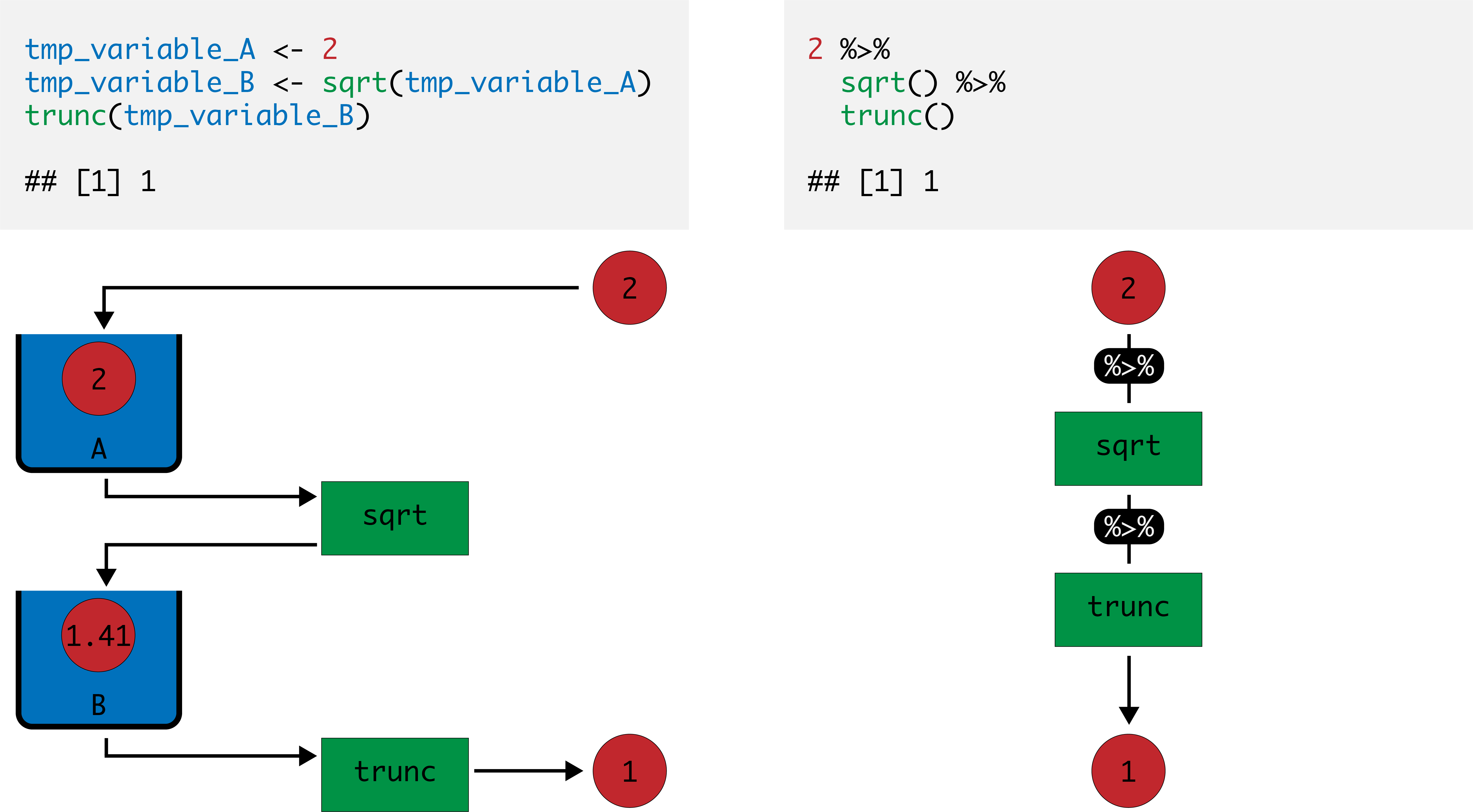
The code below shows a simple example. The number 2 is taken as input for the first pipe that passes it on as the first argument to the function sqrt. The output value 1.41 is then taken as input for the second pipe, that passes it on as the first argument to the function trunc. The final output 1 is finally returned.

2 %>%
  sqrt() %>%
  trunc()

## [1] 1

The image below graphically illustrates how the pipe operator works, compared to the same procedure executed using two temporary variables that are used to store temporary values.

sqrt(2) %>%
 round(digits = 2)

The first step of a sequence of pipes can be a value, a variable, or a function including arguments. The code below shows a series of examples a verious different ways of achieving the same result. The examples use the function round, which also allows for a second argument digits = 2. Note that, when using the pipe operator, only the nominally second argument is provided to the function round – that is round(digits = 2)

# No pipe, using variables
tmp_variable_A <- 2
tmp_variable_B <- sqrt(tmp_variable_A)
round(tmp_variable_B, digits = 2)

# No pipe, using functions only
round(sqrt(2), digits = 2)

# Pipe starting from a value
2 %>%
  sqrt() %>%
  round(digits = 2)

# Pipe starting from a variable
the_value_two <- 2
the_value_two %>%
  sqrt() %>%
  round(digits = 2)

# Pipe starting from a function
sqrt(2) %>%
 round(digits = 2)

A complex operation created through the use of %>% can be used on the right side of <-, to assign the outcome of the operation to a variable.

sqrt_of_two <- 2 %>%
  sqrt() %>%
  round(digits = 2)

1.6 Coding style

Study the Tidyverse Style Guide (style.tidyverse.org) and use it consistently!

1.7 Exercise 1.1

Question 1.1.1: Write a piece of code using the pipe operator that takes as input the number 1632, calculates the logarithm to the base 10, takes the highest integer number lower than the calculated value (lower round), and verifies whether it is an integer.

Question 1.1.2: Write a piece of code using the pipe operator that takes as input the number 1632, calculates the square root, takes the lowest integer number higher than the calculated value (higher round), and verifies whether it is an integer.

Question 1.1.3: Write a piece of code using the pipe operator that takes as input the string "1632", transforms it into a number, and checks whether the result is Not a Number.

Question 1.1.4: Write a piece of code using the pipe operator that takes as input the string "-16.32", transforms it into a number, takes the absolute value and truncates it, and finally checks whether the result is Not Available.

1.8 Exercise 1.2

Answer the question below, consulting the stringr library reference (stringr.tidyverse.org/reference) as necessary

Question 1.2.1: Write a piece of code using the pipe operator and the stringr library that takes as input the string "I like programming in R", and transforms it all in uppercase.

Question 1.2.2: Write a piece of code using the pipe operator and the stringr library that takes as input the string "I like programming in R", and truncates it, leaving only 10 characters.

Question 1.2.3: Write a piece of code using the pipe operator and the stringr library that takes as input the string "I like programming in R", and truncates it, leaving only 10 characters and using no ellipsis.

Question 1.2.4: Write a piece of code using the pipe operator and the stringr library that takes as input the string "I like programming in R", and manipulates to leave only the string "I like R".