6 Reproducibility
This work is licensed under the GNU General Public License v3.0. Contains public sector information licensed under the Open Government Licence v3.0.
6.1 Markdown
A essential tool used in creating these materials is RMarkdown That is an R library that allows you to create scripts that mix the Markdown mark-up language and R, to create dynamic documents. RMarkdown script can be compiled, at which point, the Markdown notation is interpreted to create the output files, while the R code is executed and the output incorporated in the document.
For instance the following markdown code
[This is a link to the University of Leicester](http://le.ac.uk) and **this is in bold**.is rendered as
This is a link to the University of Leicester and this is in bold.
The core Markdown notation used in this session is presented below. A full RMarkdown cheatsheet is available here.
# Header 1
## Header 2
### Header 3
#### Header 4
##### Header 5

**bold**
*italics*

[This is a link to the University of Leicester](http://le.ac.uk)

- Example list
    - Main folder
        - Analysis
        - Data
        - Utils
    - Other bullet point
- And so on
    - and so forth

1. These are
    1. Numeric bullet points
    2. Number two
2. Another number two
3. This is number three
6.1.1 R Markdown
R code can be embedded in RMarkdown documents as in the example below. That results in the code chunk be displayed within the document (as echo=TRUE is specified), followed by the output from the execution of the same code.
```{r, echo=TRUE}
a_number <- 0
a_number <- a_number + 1
a_number <- a_number + 1
a_number <- a_number + 1
a_number
```## [1] 36.2 Exercise 5.1
Create a new R project named Practical_301 as the directory name. Create an RMarkdown document in RStudio by selecting File > New File > R Markdown … – this might prompt RStudio to update some packages. On the RMarkdown document creation menu, specify “Practical 05” as title and your name as the author, and select PDF as default output format.
The new document should contain the core document information, as in the example below, plus some additional content that simply explains how RMarkdown works.
---
title: "Practical 05"
author: "A. Student"
date: "7 October 2018"
output: pdf_document
---
Delete the contents below the document information and copy the following text below the document information.
# Pipe example

This is my first [RMarkdown](https://rmarkdown.rstudio.com/) document.

```{r, echo=TRUE}
library(tidyverse)
```

The code uses the pipe operator:

- takes 2 as input
- calculates the square root
- rounds the value
    - keeping only two digits

```{r, echo=TRUE}
2 %>%
  sqrt() %>%
  round(digits = 2)
```
The option echo=TRUE tells RStudio to include the code in the output document, along with the output of the computation. If echo=FALSE is specified, the code will be omitted. If the option message=FALSE and warning=FALSE are added, messages and warnings from R are not displayed in the output document.
Save the document by selecting File > Save from the main menu. Enter Square_root as file name and click Save. The file is saved using the Rmd (RMarkdown) extension.
Click on the Knit button on the bar above the editor panel (top-left area) in RStudio, on the left side. Check the resulting pdf document. Try adding some of your own code (e.g., using some of the examples above) and Markdown text, and compile the document again.
6.3 Exercise 5.2
Create an analysis document based on RMarkdown for each one of the two analyses seen in the practical sessions 3 and 4. For each of the two analyses, within their respective R projects, first, create an RMarkdown document. Then, add the code from the related R script. Finally add additional content such as title, subtitles, and most importantly, some text describing the data used, how the analysis has been done, and the result obtained. Make sure you add appropriate links to the data sources, as available in the practical session materials.
6.4 Git
Git is a free and opensource version control system. It is commonly used through a server, where a master copy of a project is kept, but it can also be used locally. Git allows storing versions of a project, thus providing file synchronisation, consistency, history browsing, and the creation of multiple branches. For a detailed introduction to Git, please refer to the Pro Git book, written by Scott Chacon and Ben Straub.
As illustrated in the image below, when working with a git repository, the most common approach is to first check-out the latest version from the main repository before start working on any file. Once a series of edits have been made, the edits to stage are selected and then committed in a permanent snapshot. One or more commits can then be pushed to the main repository.
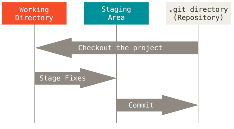
by Scott Chacon and Ben Straub, licensed under CC BY-NC-SA 3.0
6.4.1 Git and RStudio
In RStudio Server, in the Files tab of the bottom-left panel, click on Home to make sure you are in your home folder – if you are working on your own computer, create a folder for granolarr wherever most convenient. Click on New Folder and enter Repos (short for repositories) in the prompt dialogue, to create a folder named Repos.
Create a GitHub account at github.com, if you don’t have one, and create a new repository named my-granolarr, following the instructions available on the GitHub help pages. Make sure you tick the box next to Initialize this repository with a README, which adds a README.md markdown file to your repository.
Once the repository has been created, GitHub will take you to the repository page. Copy the link to the repository .git file by clicking on the green Clone or download button and copying the https URL there available. Back to RStudio Server, select File > New Project… from the top menu and select Version Control and then Git from the New Project panel. Paste the copied URL in the Repository URL field, select the Repos folder created above as folder for Create project as subdirectory of, and click Create Project. RStudio might ask you for your GitHub username and password at this point.
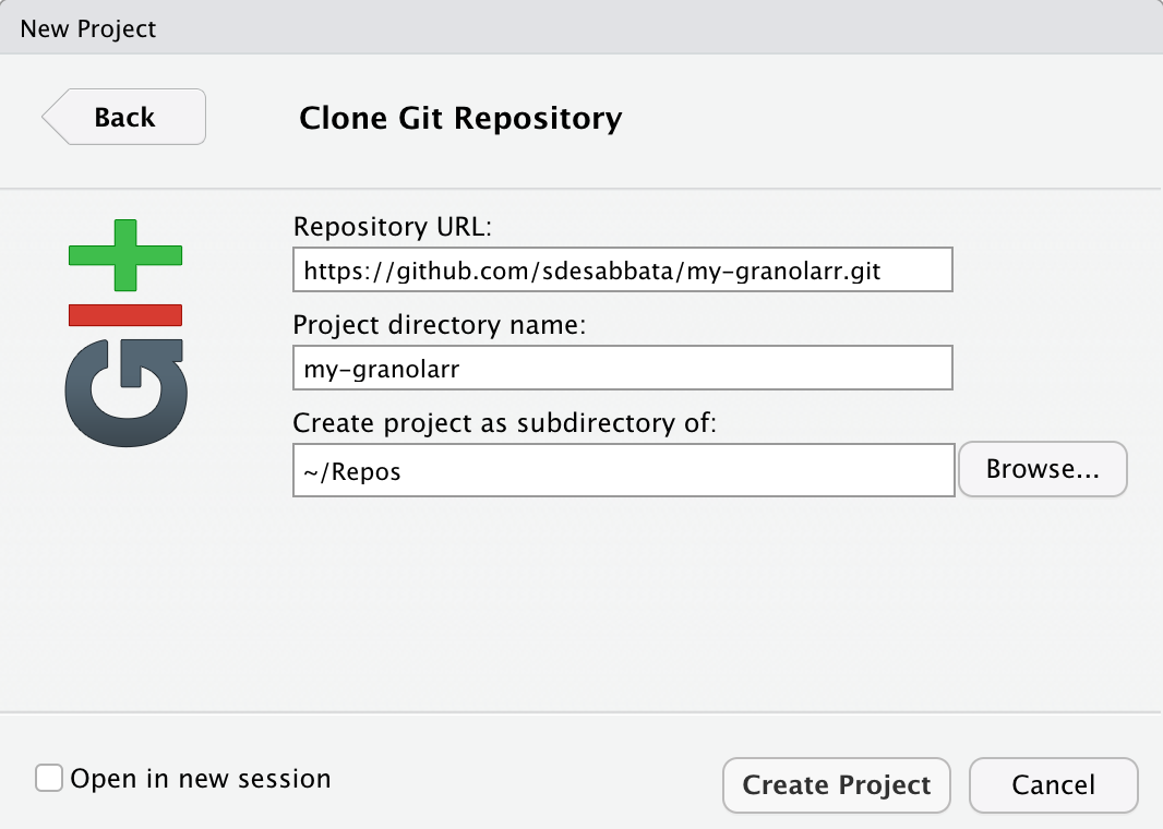
Cloning my-granolarr as R project in RStudio
Before continuing, you need to record your identity with the Git system installed on the RStudio Server, for it to be able to communicate with the GitHub’s server. Open the Terminal tab in RStudio (if not visible, select Tools > Terminal > New Terminal from the top menu). First, paste the command below substituting you@example.com with your university email (make sure to maintain the double quotes) and press the return button.
git config --global user.email "you@example.com"Then, paste the command below substituting Your Name with your name (make sure to maintain the double quotes) and press the return button.
git config --global user.name "Your Name"RStudio should have now switched to a new R project linked to you my-granolarr repository. In the RStudio File tab in the bottom-right panel, navigate to the file created for the exercises above, select the files and copy them in the folder of the new project (in the File tab, More > Copy To…).
Check the now available Git tab on the top-right panel, and you should see at least the newly copied files marked as untracked. Tick the checkboxes in the Staged column to stage the files, then click on the Commit button.
In the newly opened panel Commit window, the top-left section shows the files, and the bottom section shows the edits. Write My first commit in the Commit message section in the top-right, and click the Commit button. A pop-up should notify the completed commit. Close both the pop-up panel, and click the Push button on the top-right of the Commit window. Another pop-up panel should ask you for your GitHub username and password and then show the executed push operation. Close both the pop-up panel and the Commit window.
Congratulations, you have completed your first commit! Check the repository page on GitHub. If you reload the page, the top bar should show 2 commits on the left and your files should now be visible in the file list below. If you click on 2 commits, you can see the commit history, including both the initial commit that created the repository and the commit you just completed.
6.4.2 Cloning granolarr
You can follow the steps listed below to clone the granolarr repository.
Create a folder named
Reposin your home directory. If you are working on RStudio Server, in the Files panel, click on theHomebutton (second bar, next to the house icon), then click onNew Folder, enter the nameReposand clickOk.In RStudio or RStudio Server select
File > New Project...Select
Version Controland thenGit(you might need to set up Git first if you are working on your own computer)Copy
https://github.com/sdesabbata/granolarr.gitin theRepository URLfield and select the Repos folder for the fieldCreate project as subdirectory of, and click onCreate Project.Have a look around
Click on the project name
granolarron the top-left of the interface and selectClose Projectto close the project.
As granolarr is a public repository, you can clone it, edit it as you wish and push it to your own copy of the repository. However, contributing your edits to the original repository would require a few further steps. Check out the GitHub help pages if you are interested.
6.5 Exercise 5.3
Create a new repository for an R project exploring the presence of the different living arrangements in Leicester among both the different categories of the 2011 Output Area Classification and deciles of Index of Multiple Deprivations. Create the repository, clone it to RStudio Server as a new R project, and copy the required data in the project folder. Create an RMarkdown document and write your analysis, including:
- an introduction to the data and the aims of the project;
- a justification of the analysis methods;
- the code and related results;
- and a discussion of the results within the same document.