8 Regression analysis

Stefano De Sabbata

This work is licensed under the GNU General Public License v3.0. Contains public sector information licensed under the Open Government Licence v3.0.

8.1 Introduction

The first part of this practical guides you through the ANOVA (analysis of variance) and regression analysis seen in the lecture, the last part showcases a multiple regression analysis. Create a new R project for this practical session and create a new RMarkdown document to replicate the analysis in this document and a separate RMarkdown document to work on the exercises.

library(tidyverse)
library(magrittr)
library(knitr)

Many of the functions used in the analyses below are part of the oldest libraries developed for R, they have not been developed to be easily compatible with the Tidyverse and the %>% operator. Fortunately, the magrittr library (loaded above) does not only define the %>% operator seen so far, but also the exposition pipe operator %$%, which exposes the columns of the data.frame on the left of the operator to the expression on the right of the operator. That is, %$% allows to refer to the column of the data.frame directly in the subsequent expression. As such, the lines below expose the column Petal.Length of the data.frame iris and to pass it on to the mean function using different approaches, but they are all equivalent in their outcome.

mean(iris$Petal.Length) # Classic R approach

## [1] 3.758

iris$Petal.Length %>% mean() # Using %>% pipe

## [1] 3.758

iris %$% Petal.Length %>% mean() # Using %>% pipe and %$% exposition pipe

## [1] 3.758

8.2 ANOVA

The ANOVA (analysis of variance) tests whether the values of a variable (e.g., length of the petal) are on average different for different groups (e.g., different species of iris). ANOVA has been developed as a generalised version of the t-test, which has the same objective but allows to test only two groups.

The ANOVA test has the following assumptions:

normally distributed values in groups
- especially if groups have different sizes
homogeneity of variance of values in groups
- if groups have different sizes
independence of groups

8.2.1 Example

The example seen in the lecture illustrates how ANOVA can be used to verify that the three different species of iris in the iris dataset have different petal length.

iris %>%
  ggplot(
    aes(
      x = Species, 
      y = Petal.Length
    )
  ) +
  geom_boxplot()

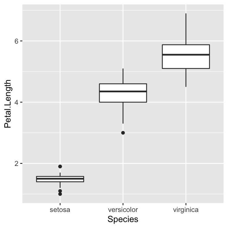
ANOVA is considered a robust test, thus, as the groups are of the same size, there is no need to test for the homogeneity of variance. Furthermore, the groups come from different species of flowers, so there is no need to test the independence of the values. The only assumption that needs testing is whether the values in the three groups are normally distributed. The three Shapiro–Wilk tests below are all not significant, which indicates that all three groups have normally distributed values.

iris %>% filter(Species == "setosa") %>% pull(Petal.Length) %>% shapiro.test()

## 
##  Shapiro-Wilk normality test
## 
## data:  .
## W = 0.95498, p-value = 0.05481

iris %>% filter(Species == "versicolor") %>% pull(Petal.Length) %>% shapiro.test()

## 
##  Shapiro-Wilk normality test
## 
## data:  .
## W = 0.966, p-value = 0.1585

iris %>% filter(Species == "virginica") %>% pull(Petal.Length) %>% shapiro.test()

## 
##  Shapiro-Wilk normality test
## 
## data:  .
## W = 0.96219, p-value = 0.1098

We can thus conduct the ANOVA test using the function aov, and the function summary to obtain the summary of the results of the test.

# Classic R coding approach (not using %$%)
# iris_anova <- aov(Petal.Length ~ Species, data = iris)
# summary(iris_anova)

iris %$%
  aov(Petal.Length ~ Species) %>%
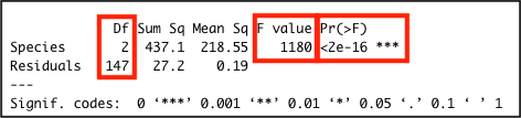
  summary()

##              Df Sum Sq Mean Sq F value Pr(>F)    
## Species       2  437.1  218.55    1180 <2e-16 ***
## Residuals   147   27.2    0.19                   
## ---
## Signif. codes:  0 '***' 0.001 '**' 0.01 '*' 0.05 '.' 0.1 ' ' 1

The difference is significant F(2, 147) = 1180.16, p < .01.

The image below highlights the important values in the output: the significance value Pr(>F); the F-statistic value F value; and the two degrees of freedom values for the F-statistic in the Df column.

8.3 Simple regression

The simple regression analysis is a supervised machine learning approach to creating a model able to predict the value of one outcome variable $Y$ based on one predictor variable $X_1$, by estimating the intercept $b_0$ and coefficient (slope) $b_1$, and accounting for a reasonable amount of error $\epsilon$.

\[Y_i = (b_0 + b_1 * X_{i1}) + \epsilon_i \]

Least squares is the most commonly used approach to generate a regression model. This model fits a line to minimise the squared values of the residuals (errors), which are calculated as the squared difference between observed values the values predicted by the model.

\[redidual = \sum(observed - model)^2\]

A model is considered robust if the residuals do not show particular trends, which would indicate that “something” is interfering with the model. In particular, the assumption of the regression model are:

linearity: the relationship is actually linear;
normality of residuals: standard residuals are normally distributed with mean 0;
homoscedasticity of residuals: at each level of the predictor variable(s) the variance of the standard residuals should be the same (homo-scedasticity) rather than different (hetero-scedasticity);
independence of residuals: adjacent standard residuals are not correlated.

8.3.1 Example

The example that we have seen in the lecture illustrated how simple regression can be used to create a model to predict the arrival delay based on the departure delay of a flight, based on the data available in the nycflights13 dataset for the flight on November 20th, 2013. The scatterplot below seems to indicate that the relationship is indeed linear.

\[arr\_delay_i = (Intercept + Coefficient_{dep\_delay} * dep\_delay_{i1}) + \epsilon_i \]

# Load the library
library(nycflights13)

# November 20th, 2013
flights_nov_20 <- nycflights13::flights %>%
  filter(!is.na(dep_delay), !is.na(arr_delay), month == 11, day ==20)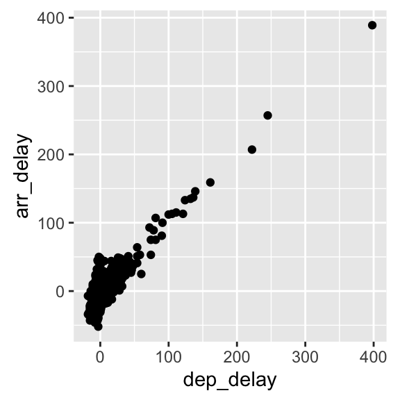

The code below generates the model using the function lm, and the function summary to obtain the summary of the results of the test. The model and summary are saved in the variables delay_model and delay_model_summary, respectively, for further use below. The variable delay_model_summary can then be called directly to visualise the result of the test.

# Classic R coding version
# delay_model <- lm(arr_delay ~ dep_delay, data = flights_nov_20)
# delay_model_summary <- summary(delay_model)

delay_model <- flights_nov_20 %$%
  lm(arr_delay ~ dep_delay) 

delay_model_summary <- delay_model %>%
  summary()

delay_model_summary

## 
## Call:
## lm(formula = arr_delay ~ dep_delay)
## 
## Residuals:
##     Min      1Q  Median      3Q     Max 
## -43.906  -9.022  -1.758   8.678  57.052 
## 
## Coefficients:
##             Estimate Std. Error t value Pr(>|t|)    
## (Intercept) -4.96717    0.43748  -11.35   <2e-16 ***
## dep_delay    1.04229    0.01788   58.28   <2e-16 ***
## ---
## Signif. codes:  0 '***' 0.001 '**' 0.01 '*' 0.05 '.' 0.1 ' ' 1
## 
## Residual standard error: 13.62 on 972 degrees of freedom
## Multiple R-squared:  0.7775, Adjusted R-squared:  0.7773 
## F-statistic:  3397 on 1 and 972 DF,  p-value: < 2.2e-16

The image below highlights the important values in the output: the adjusted $R^2$ value; the model significance value p-value and the related F-statistic information F-statistic; the intercept and dep_delay coefficient estimates in the Estimate column and the related significance values of in the column Pr(>|t|).

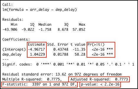
The output indicates:

p-value: < 2.2e-16: $p<.001$ the model is significant;
- derived by comparing the calulated F-statistic value to F distribution 3396.74 having specified degrees of freedom (1, 972);
- Report as: $F(1, 972) = 3396.74$
Adjusted R-squared: 0.7773: the departure delay can account for 77.73% of the arrival delay;
Coefficients:
- Intercept estimate -4.9672 is significant;
- dep_delay coefficient (slope) estimate 1.0423 is significant.

flights_nov_20 %>%
  ggplot(aes(x = dep_delay, y = arr_delay)) +
  geom_point() + coord_fixed(ratio = 1) +
  geom_abline(intercept = 4.0943, slope = 1.04229, color="red")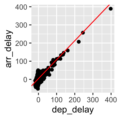

8.3.2 Checking assumptions

8.3.2.1 Normality

The Shapiro-Wilk test can be used to check for the normality of standard residuals. The test should be not significant for robust models. In the example below, the standard residuals are not normally distributed. However, the plot further below does show that the distribution of the residuals is not far away from a normal distribution.

delay_model %>% 
  rstandard() %>% 
  shapiro.test()

## 
##  Shapiro-Wilk normality test
## 
## data:  .
## W = 0.98231, p-value = 1.73e-09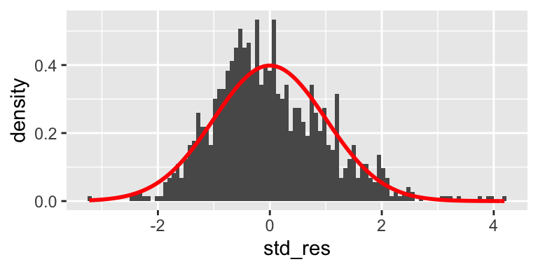

8.3.2.2 Homoscedasticity

The Breusch-Pagan test can be used to check for the homoscedasticity of standard residuals. The test should be not significant for robust models. In the example below, the standard residuals are homoscedastic.

library(lmtest)

delay_model %>% 
  bptest()

## 
##  studentized Breusch-Pagan test
## 
## data:  .
## BP = 0.017316, df = 1, p-value = 0.8953

8.3.2.3 Independence

The Durbin-Watson test can be used to check for the independence of residuals. The test should be statistic should be close to 2 (between 1 and 3) and not significant for robust models. In the example below, the standard residuals might not be completely independent. Note, however, that the result depends on the order of the data.

# Also part of the library lmtest
delay_model %>%
  dwtest()

## 
##  Durbin-Watson test
## 
## data:  .
## DW = 1.8731, p-value = 0.02358
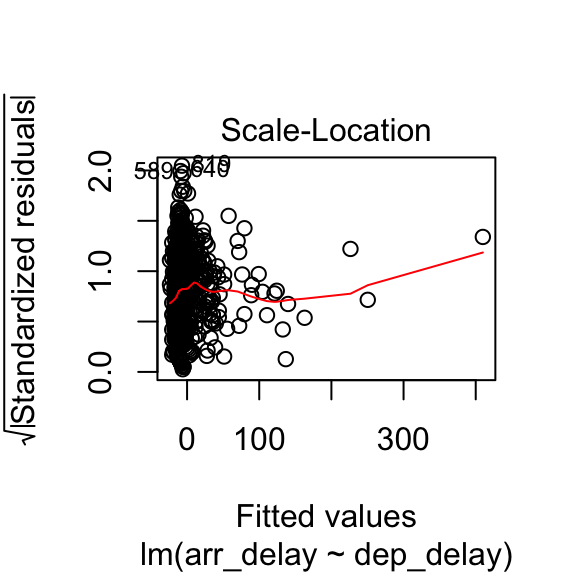
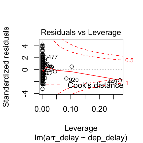
## alternative hypothesis: true autocorrelation is greater than 0

8.3.2.4 Plots

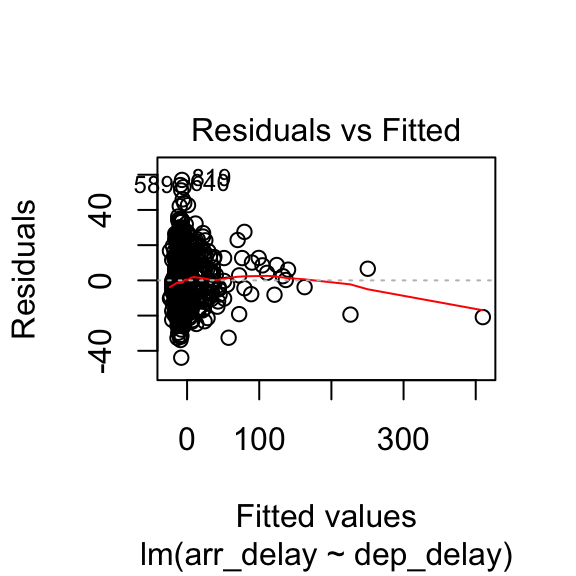
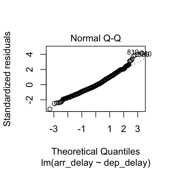
The plot.lm function can be used to further explore the residuals visuallly. Usage is illustrated below. The Residuals vs Fitted and Scale-Location plot provide an insight into the homoscedasticity of the residuals, the Normal Q-Q plot provides an illustration of the normality of the residuals, and the Residuals vs Leverage can be useful to identify exceptional cases (e.g., Cook’s distance greater than 1).

delay_model %>%
  plot()

8.3.3 How to report

Overall, we can say that the delay model computed above is fit ($F(1, 972) = 3396.74$, $p < .001$), indicating that the departure delay might account for 77.73% of the arrival delay. However the model is only partially robust. The residuals satisfy the homoscedasticity assumption (Breusch-Pagan test, $BP = 0.02$, $p =0.9$), and the independence assumption (Durbin-Watson test, $DW = 1.87$, $p =0.02$), but they are not normally distributed (Shapiro-Wilk test, $W = 0.98$, $p < .001$).

The stargazer function of the stargazer library can be applied to the model delay_model to generate a nicer output in RMarkdown PDF documents by including results = "asis" in the R snippet option.

# Install stargazer if not yet installed
# install.packages("stargazer")

library(stargazer)

# Not rendered in bookdown
stargazer(delay_model)

% Table created by stargazer v.5.2.2 by Marek Hlavac, Harvard University. E-mail: hlavac at fas.harvard.edu % Date and time: Wed, Jan 15, 2020 - 00:38:17

8.4 Multiple regression

The multiple regression analysis is a supervised machine learning approach to creating a model able to predict the value of one outcome variable $Y$ based on two or more predictor variables $X_1 \dots X_M$, by estimating the intercept $b_0$ and the coefficients (slopes) $b_1 \dots b_M$, and accounting for a reasonable amount of error $\epsilon$.

\[Y_i = (b_0 + b_1 * X_{i1} + b_2 * X_{i2} + \dots + b_M * X_{iM}) + \epsilon_i \]

The assumptions are the same as the simple regression, plus the assumption of no multicollinearity: if two or more predictor variables are used in the model, each pair of variables not correlated. This assumption can be tested by checking the variance inflation factor (VIF). If the largest VIF value is greater than 10 or the average VIF is substantially greater than 1, there might be an issue of multicollinearity.

8.4.1 Example

The example below explores whether a regression model can be created to estimate the number of people in Leicester commuting to work using public transport (u120) in Leicester, using the number of people in different occupations as predictors.

For instance, occupations such as skilled traders usually require to travel some distances with equipment, thus the related variable u163 is not included in the model, whereas professional and administrative occupations might be more likely to use public transportation to commute to work.

A multiple regression model can be specified in a similar way as a simple regression model, using the same lm function, but adding the additional predictor variables using a + operator.

leicester_2011OAC <- read_csv("2011_OAC_Raw_uVariables_Leicester.csv")

# u120: Method of Travel to Work, Public Transport
# u159: Employment, Managers, directors and senior officials
# u160: Employment, Professional occupations
# u161: Employment, Associate professional and technical occupations
# u162: Employment, Administrative and secretarial occupations
# u163: Employment, Skilled trades occupations
# u164: Employment, Caring, leisure and other service occupations
# u165: Employment, Sales and customer service occupations
# u166: Employment, Process, plant and machine operatives
# u167: Employment, Elementary occupations
public_transp_model <- leicester_2011OAC %$%
  lm(u120 ~ u160 + u162 + u164 + u165 + u167) 

public_transp_model %>%
  summary()

## 
## Call:
## lm(formula = u120 ~ u160 + u162 + u164 + u165 + u167)
## 
## Residuals:
##      Min       1Q   Median       3Q      Max 
## -16.8606  -4.0247  -0.1084   3.7912  24.6359 
## 
## Coefficients:
##             Estimate Std. Error t value Pr(>|t|)    
## (Intercept)  3.19593    0.75048   4.258 2.26e-05 ***
## u160         0.06912    0.01416   4.881 1.24e-06 ***
## u162         0.17000    0.03328   5.108 3.93e-07 ***
## u164         0.28641    0.03589   7.979 4.17e-15 ***
## u165         0.21311    0.03107   6.858 1.25e-11 ***
## u167         0.32008    0.02156  14.846  < 2e-16 ***
## ---
## Signif. codes:  0 '***' 0.001 '**' 0.01 '*' 0.05 '.' 0.1 ' ' 1
## 
## Residual standard error: 5.977 on 963 degrees of freedom
## Multiple R-squared:  0.436,  Adjusted R-squared:  0.4331 
## F-statistic: 148.9 on 5 and 963 DF,  p-value: < 2.2e-16

# Not rendered in bookdown
stargazer(public_transp_model)

% Table created by stargazer v.5.2.2 by Marek Hlavac, Harvard University. E-mail: hlavac at fas.harvard.edu % Date and time: Wed, Jan 15, 2020 - 00:38:17

public_transp_model %>%
  rstandard() %>% 
  shapiro.test()

## 
##  Shapiro-Wilk normality test
## 
## data:  .
## W = 0.9969, p-value = 0.05628

public_transp_model %>% 
  bptest()

## 
##  studentized Breusch-Pagan test
## 
## data:  .
## BP = 45.986, df = 5, p-value = 9.142e-09

public_transp_model %>%
  dwtest()

## 
##  Durbin-Watson test
## 
## data:  .
## DW = 1.8463, p-value = 0.007967
## alternative hypothesis: true autocorrelation is greater than 0

library(car)

public_transp_model %>%
  vif()

##     u160     u162     u164     u165     u167 
## 1.405480 1.486768 1.163760 1.353682 1.428418

The output above suggests that the model is fit ($F(5, 963) = 148.88$, $p < .001$), indicating that a model based on the number of people working in the five selected occupations can account for 43.31% of the number of people using public transportation to commute to work. However the model is only partially robust. The residuals are normally distributed (Shapiro-Wilk test, $W = 1$, $p =0.06$) and there seems to be no multicollinearity with average VIF $1.37$, but the residuals don’t satisfy the homoscedasticity assumption (Breusch-Pagan test, $BP = 45.99$, $p < .001$), nor the independence assumption (Durbin-Watson test, $DW = 1.85$, $p < .01$).

The coefficient values calculated by the lm functions are important to create the model, and provide useful information. For instance, the coefficient for the variable u165 is 0.21, which indicates that if the number of people employed in sales and customer service occupations increases by one unit, the number of people using public transportation to commute to work increases by 0.21 units, according to the model. The coefficients also indicate that the number of people in elementary occupations has the biggest impact (in the context of the variables selected for the model) on the number of people using public transportation to commute to wor0, whereas the number of people in professional occupations has the lowest impact.

In this example, all variables use the same unit and are of a similar type, which makes interpretating the model relatively simple. When that is not the case, it can be useful to look at the standardized $\beta$, which provide the same information but measured in terms of standard deviation, which make comparisons between variables of different types easier to draw. For instance, the values calculated below using the function lm.beta of the library QuantPsyc indicate that if the number of people employed in sales and customer service occupations increases by one standard deviation, the number of people using public transportation to commute to work increases by 0.19 standard deviations, according to the model.

# Install lm.beta library if necessary
# install.packages("lm.beta")
library(lm.beta)

lm.beta(public_transp_model)

## 
## Call:
## lm(formula = u120 ~ u160 + u162 + u164 + u165 + u167)
## 
## Standardized Coefficients::
## (Intercept)        u160        u162        u164        u165        u167 
##   0.0000000   0.1400270   0.1507236   0.2083107   0.1931035   0.4293988

8.5 Exercise 9.1

Question 9.1.1: Is mean age (u020) different in different 2011OAC supergroups in Leicester?

Question 9.1.2: Is the number of people using public transportation to commute to work statistically, linearly related to mean age (u020)?

Question 9.1.3: Is the number of people using public transportation to commute to work statistically, linearly related to (a subset of) the age structure categories (u007 to u019)?