33 Exploring assumptions

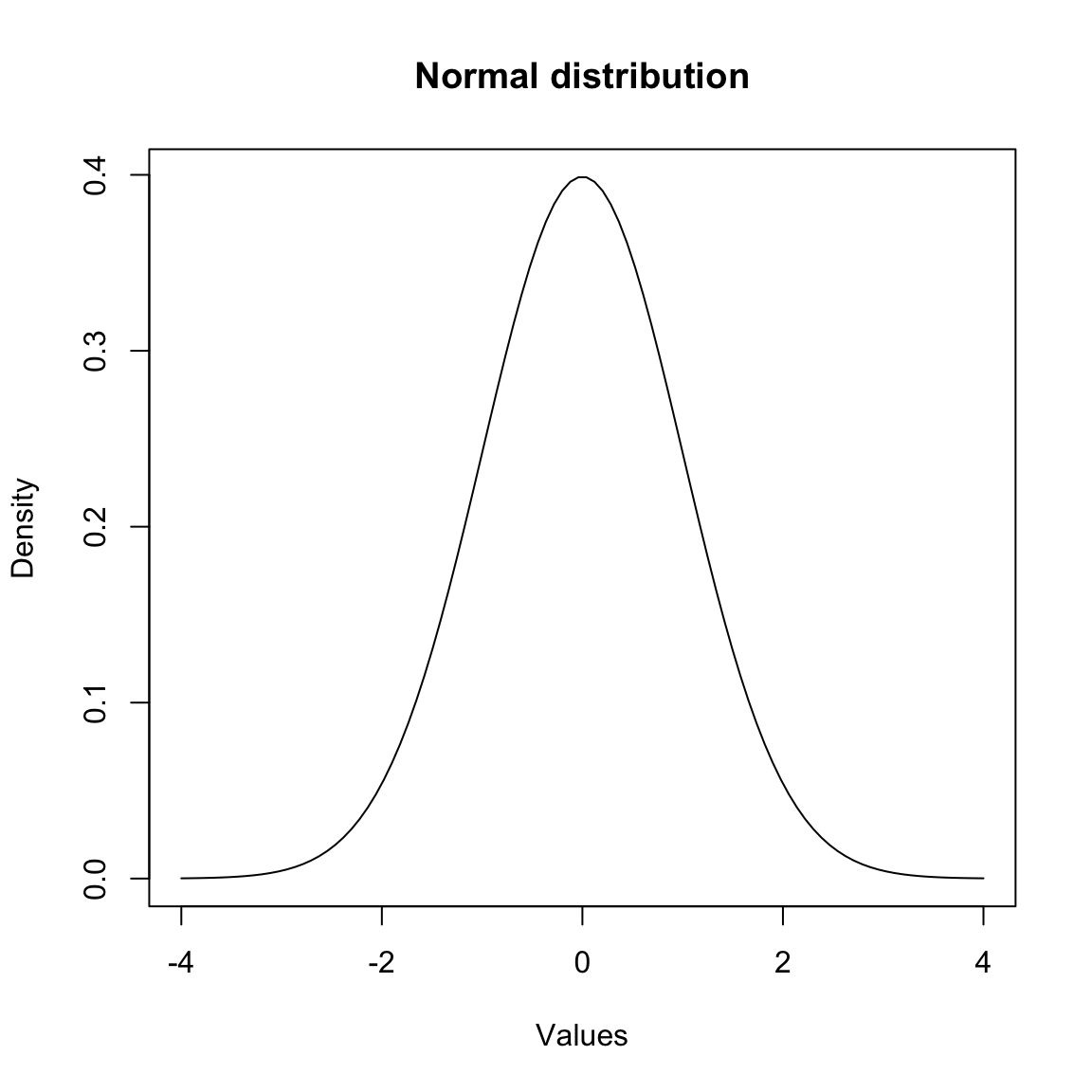
33.1 Normal distribution

• characterized by the bell-shaped curve
• majority of values lie around the centre of the distribution
• the further the values are from the centre, the lower their frequency
• about 95% of values within 2 standard deviations from the mean

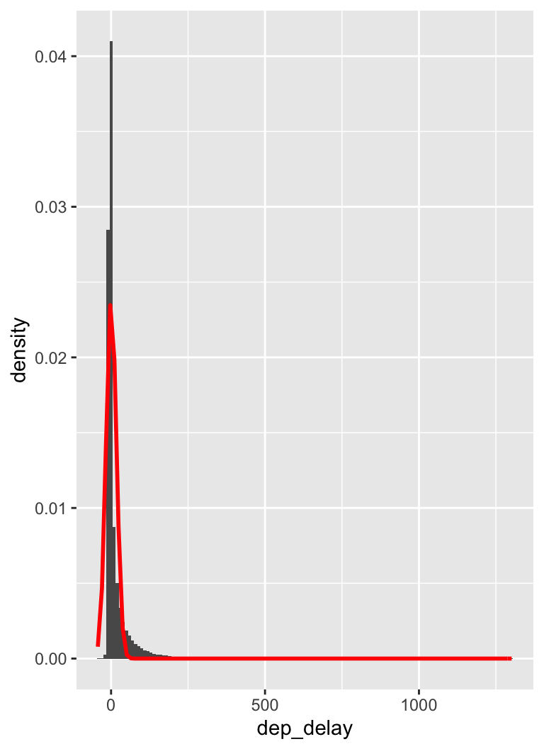
33.2 Density histogram

nycflights13::flights %>% 
  ggplot(
    aes(
      x = dep_delay
    )
  ) +
  geom_histogram(
    aes(
      y =..density..
    ),
    binwidth = 10
  ) + 
  stat_function(
    fun = dnorm, 
    args = list(
      mean = dep_delay_mean,
      sd = dep_delay_sd),
    colour = "black", size = 1)

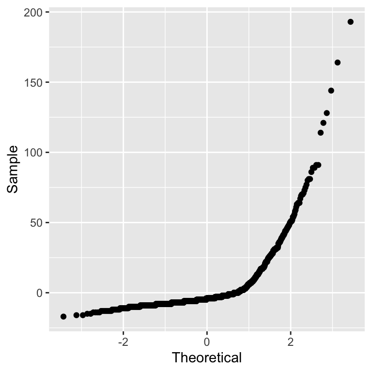
33.3 Q-Q plot

Cumulative values against the cumulative probability of a particular distribution

nycflights13::flights %>%
  filter(
    month == 11, 
    carrier == "US"
  ) %>%
  qplot(
    sample = dep_delay, 
    data = .,
    stat = "qq", 
    xlab = "Theoretical", 
    ylab = "Sample"
  )

33.4 stat.desc: norm

nycflights13::flights %>%
  filter(month == 11, carrier == "US") %>%
  select(dep_delay, arr_delay, distance) %>%
  stat.desc(basic = FALSE, desc = FALSE, norm = TRUE) %>%
  kable()

	dep_delay	arr_delay	distance
skewness	4.4187763	2.0716291	2.0030249
skew.2SE	36.8709612	17.2808242	16.8678747
kurtosis	28.8513206	9.5741004	2.6000743
kurt.2SE	120.4418092	39.9557893	10.9542887
normtest.W	0.5545326	0.8657894	0.6012442
normtest.p	0.0000000	0.0000000	0.0000000

33.5 Normality

Shapiro–Wilk test compares the distribution of a variable with a normal distribution having same mean and standard deviation

• If significant, the distribution is not normal
• normtest.W (test statistics) and normtest.p (significance)
• also, shapiro.test function is available

nycflights13::flights %>%
  filter(month == 11, carrier == "US") %>%
  pull(dep_delay) %>%
  shapiro.test()

## 
##  Shapiro-Wilk normality test
## 
## data:  .
## W = 0.55453, p-value < 2.2e-16

33.6 Significance

Most statistical tests are based on the idea of hypothesis testing

• a null hypothesis is set
• the data are fit into a statistical model
• the model is assessed with a test statistic
• the significance is the probability of obtaining that test statistic value by chance

The threshold to accept or reject an hypotheis is arbitrary and based on conventions (e.g., p < .01 or p < .05)

Example: The null hypotheis of the Shapiro–Wilk test is that the sample is normally distributed and p < .01 indicates that the probability of that being true is very low.

33.7 Skewness and kurtosis

In a normal distribution, the values of skewness and kurtosis should be zero

• skewness: skewness value indicates
  • positive: the distribution is skewed towards the left
  • negative: the distribution is skewed towards the right
• kurtosis: kurtosis value indicates
  • positive: heavy-tailed distribution
  • negative: flat distribution
• skew.2SE and kurt.2SE: skewness and kurtosis divided by 2 standard errors. If greater than 1, the respective statistics is significant (p < .05).

33.8 Homogeneity of variance

Levene’s test for equality of variance in different levels

• If significant, the variance is different in different levels

dep_delay_carrier <- nycflights13::flights %>%
  filter(month == 11) %>%
  select(dep_delay, carrier)

library(car)
leveneTest(dep_delay_carrier$dep_delay, dep_delay_carrier$carrier)

## Levene's Test for Homogeneity of Variance (center = median)
##          Df F value    Pr(>F)    
## group    15  20.203 < 2.2e-16 ***
##       27019                      
## ---
## Signif. codes:  0 '***' 0.001 '**' 0.01 '*' 0.05 '.' 0.1 ' ' 1