38 Lecture 502
Regression

38.1 Regression analysis

Regression analysis is a supervised machine learning approach

Predict the value of one outcome variable as

\[outcome_i = (model) + error_i \]

one predictor variable (simple / univariate regression)

\[Y_i = (b_0 + b_1 * X_{i1}) + \epsilon_i \]

more predictor variables (multiple / multivariate regression)

\[Y_i = (b_0 + b_1 * X_{i1} + b_2 * X_{i2} + \dots + b_M * X_{iM}) + \epsilon_i \]

38.2 Least squares

Least squares is the most commonly used approach to generate a regression model

The model fits a line

to minimise the squared values of the residuals (errors)
that is squared difference between
- observed values
- model

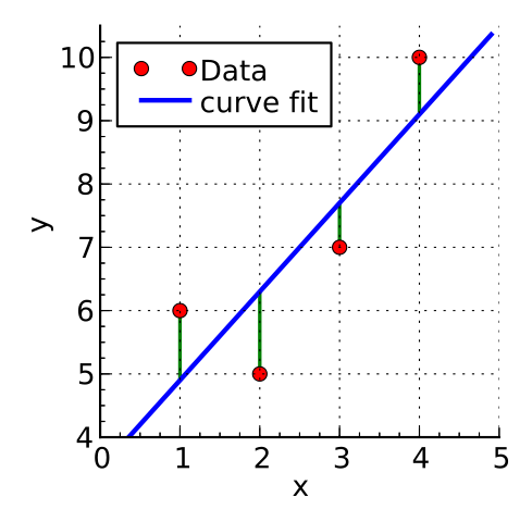
by Krishnavedala
via Wikimedia Commons,
CC-BY-SA-3.0

\[deviation = \sum(observed - model)^2\]

38.3 Example

\[arr\_delay_i = (b_0 + b_1 * dep\_delay_{i1}) + \epsilon_i \]

delay_model <- flights_nov_20 %$% # Note %$%
  lm(arr_delay ~ dep_delay)

delay_model %>%  summary()

## 
## Call:
## lm(formula = arr_delay ~ dep_delay)
## 
## Residuals:
##     Min      1Q  Median      3Q     Max 
## -43.906  -9.022  -1.758   8.678  57.052 
## 
## Coefficients:
##             Estimate Std. Error t value Pr(>|t|)    
## (Intercept) -4.96717    0.43748  -11.35   <2e-16 ***
## dep_delay    1.04229    0.01788   58.28   <2e-16 ***
## ---
## Signif. codes:  0 '***' 0.001 '**' 0.01 '*' 0.05 '.' 0.1 ' ' 1
## 
## Residual standard error: 13.62 on 972 degrees of freedom
## Multiple R-squared:  0.7775, Adjusted R-squared:  0.7773 
## F-statistic:  3397 on 1 and 972 DF,  p-value: < 2.2e-16

38.4 Overall fit

The output indicates

p-value: < 2.2e-16: \(p<.001\) the model is significant
- derived by comparing the calulated F-statistic value to F distribution 3396.74 having specified degrees of freedom (1, 972)
- Report as: F(1, 972) = 3396.74
Adjusted R-squared: 0.7773: the departure delay can account for 77.73% of the arrival delay
Coefficients
- Intercept estimate -4.9672 is significant
- dep_delay (slope) estimate 1.0423 is significant

38.5 Parameters

\[arr\_delay_i = (Intercept + Coefficient_{dep\_delay} * dep\_delay_{i1}) + \epsilon_i \]

flights_nov_20 %>%
  ggplot(aes(x = dep_delay, y = arr_delay)) +
  geom_point() + coord_fixed(ratio = 1) +
  geom_abline(intercept = 4.0943, slope = 1.04229, color="red")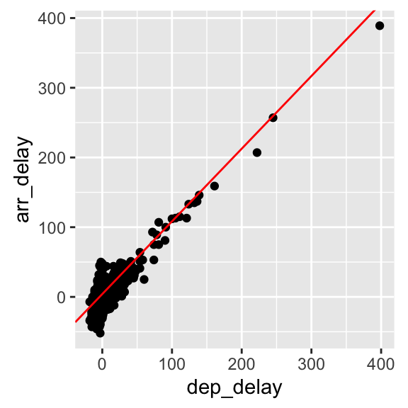

38.6 Checking assumptions

Linearity
- the relationship is actually linear
Normality of residuals
- standard residuals are normally distributed with mean 0
Homoscedasticity of residuals
- at each level of the predictor variable(s) the variance of the standard residuals should be the same (homo-scedasticity) rather than different (hetero-scedasticity)
Independence of residuals
- adjacent standard residuals are not correlated
When more than one predictor: no multicollinearity
- if two or more predictor variables are used in the model, each pair of variables not correlated

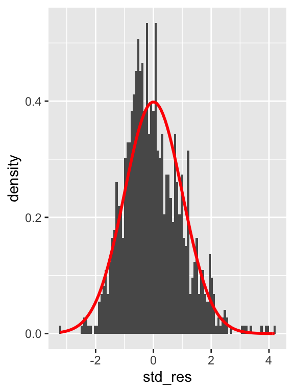
38.7 Normality

Shapiro-Wilk test for normality of standard residuals,

robust models: should be not significant

delay_model %>% 
  rstandard() %>% 
  shapiro.test()

## 
##  Shapiro-Wilk normality test
## 
## data:  .
## W = 0.98231, p-value = 1.73e-09

Standard residuals are NOT normally distributed

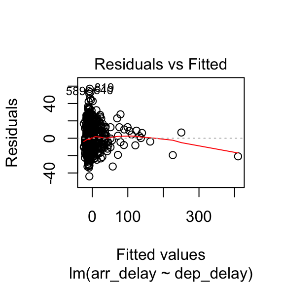
38.8 Homoscedasticity

Breusch-Pagan test for homoscedasticity of standard residuals

robust models: should be not significant

library(lmtest)

delay_model %>% 
  bptest()

## 
##  studentized Breusch-Pagan test
## 
## data:  .
## BP = 0.017316, df = 1, p-value = 0.8953

Standard residuals are homoscedastic

38.9 Independence

Durbin-Watson test for the independence of residuals

robust models: statistic should be close to 2 (between 1 and 3) and not significant

# Also part of the library lmtest
delay_model %>%
  dwtest()

## 
##  Durbin-Watson test
## 
## data:  .
## DW = 1.8731, p-value = 0.02358
## alternative hypothesis: true autocorrelation is greater than 0

Standard residuals might not be completely indipendent

Note: the result depends on the order of the data.

38 Lecture 502 Regression