6 Exploratory statistics

Print this chapter

This chapter showcases an exploratory analysis of the distribution of people aged 20 to 24 in Leicester, using the u011 variable from the 2011 Output Area Classification (2011OAC) already used in previous chapters. Before continuing, open the project created for the previous chapter. Create new RMarkdown document within that project to replicate the analysis in this document. Once the document is set up, start by adding an R code snipped including the code below, which is loads the 2011OAC dataset and the libraries used for this chapter.

library(tidyverse)
library(knitr)

leicester_2011OAC <- read_csv("2011_OAC_Raw_uVariables_Leicester.csv")

The graphics above provide preliminary evidence that the distribution of people aged 20 to 24 might, in fact, be different in different 2011 supergroups. In the remainder of the chapter, we are going to explore that hypothesis further. First, load the necessary statistical libraries.

library(pastecs)
library(car)

The code below calculates the percentage of people aged 20 to 24 (i.e., u011) over total population per OA, but it also recodes (see recode) the names of the 2011OAC supergroups to a shorter 2-letter version, which is useful for the tables presented further below. Note that the code below uses the library name as a prefix dplyr:: in front of the function name recode (thus, dplyr::recode) to make sure the function recode of the package car (thus, car::recode) is not used instead.

Only the OA code, the recoded 2011OAC supergroup name, and the newly created perc_age_20_to_24 are retained in the new table leic_2011OAC_20to24. Such a step is sometimes useful as stepping stone for further analysis and can make the code easier to read further down the line. Sometimes it is also a necessary step when interacting with certain libraries, which are not fully compatible with Tidyverse libraries, such as leveneTest (more on that function below).

leic_2011OAC_20to24 <- leicester_2011OAC %>%
  mutate(
    perc_age_20_to_24 = (u011 / Total_Population) * 100,
    supgrpname = 
      dplyr::recode(
        supgrpname, 
          `Suburbanites` = "SU",
          `Cosmopolitans` = "CP",
          `Multicultural Metropolitans` = "MM",
          `Ethnicity Central` = "EC",
          `Constrained City Dwellers` = "CD",
          `Hard-Pressed Living` = "HP",
          `Urbanites` = "UR"
    )
  ) %>%
  select(OA11CD, supgrpname, perc_age_20_to_24)

leic_2011OAC_20to24 %>%
  slice_head(n = 5) %>%
  kable()

OA11CD	supgrpname	perc_age_20_to_24
E00069517	SU	4.153355
E00069514	CP	30.650155
E00169516	MM	12.316716
E00169048	MM	6.956522
E00169044	MM	6.211180

6.1 Descriptive statistics

The first step of any statistical analysis or modelling should be to explore the “shape” of the data involved, by looking at the descriptive statistics of all variables involved. The function stat.desc of the pastecs library provides three series of descriptive statistics.

base:
- nbr.val: overall number of values in the dataset;
- nbr.null: number of NULL values – NULL is often returned by expressions and functions whose values are undefined;
- nbr.na: number of NAs – missing value indicator;
desc:
- min (see also min function): minimum value in the dataset;
- max (see also max function): minimum value in the dataset;
- range: difference between min and max (different from range());
- sum (see also sum function): sum of the values in the dataset;
- median (see also median function): median, that is the value separating the higher half from the lower half the values
- mean (see also mean function): arithmetic mean, that is sum over the number of values not NA;
- SE.mean: standard error of the mean – estimation of the variability of the mean calculated on different samples of the data (see also central limit theorem);
- CI.mean.0.95: 95% confidence interval of the mean – indicates that there is a 95% probability that the actual mean is within that distance from the sample mean;
- var: variance (\(\sigma^2\)), it quantifies the amount of variation as the average of squared distances from the mean;
- std.dev: standard deviation (\(\sigma\)), it quantifies the amount of variation as the square root of the variance;
- coef.var: variation coefficient it quantifies the amount of variation as the standard deviation divided by the mean;
norm (default is FALSE, use norm = TRUE to include it in the output):
- skewness: skewness value indicates
  - positive: the distribution is skewed towards the left;
  - negative: the distribution is skewed towards the right;
- kurtosis: kurtosis value indicates:
  - positive: heavy-tailed distribution;
  - negative: flat distribution;
- skew.2SE and kurt.2SE: skewness and kurtosis divided by 2 standard errors. If greater than 1, the respective statistics is significant (p < .05);
- normtest.W: test statistics for the Shapiro–Wilk test for normality;
- normtest.p: significance for the Shapiro–Wilk test for normality.

The Shapiro–Wilk test compares the distribution of a variable with a normal distribution having the same mean and standard deviation. The null hypothesis of the Shapiro–Wilk test is that the sample is normally distributed, thus if normtest.p is lower than 0.01 (i.e., p < .01), the test indicates that the distribution is most probably not normal. The threshold to accept or reject a hypothesis is arbitrary and based on conventions, where p < .01 is the most commonly accepted threshold, or p < .05 for relatively small data sample (e.g., 30 cases).

The next step is thus to apply the stat.desc to the variable we are currently exploring (i.e., perc_age_20_to_24), including the norm section.

leic_2011OAC_20to24_stat_desc <- leic_2011OAC_20to24 %>%
  select(perc_age_20_to_24) %>%
  stat.desc(norm = TRUE)
  
leic_2011OAC_20to24_stat_desc %>%
  kable(digits = 3)

	perc_age_20_to_24
nbr.val	969.000
nbr.null	0.000
nbr.na	0.000
min	1.064
max	60.751
range	59.687
sum	10238.502
median	7.514
mean	10.566
SE.mean	0.304
CI.mean.0.95	0.596
var	89.386
std.dev	9.454
coef.var	0.895
skewness	2.710
skew.2SE	17.249
kurtosis	7.707
kurt.2SE	24.549
normtest.W	0.645
normtest.p	0.000

The table above tells us that all 969 OA in Leicester have a valid value for the variable perc_age_20_to_24, as no NULL nor NA value have been found. The values vary from about 1% to almost 61%, with an average value of 11% of the population in an OA aged between 20 and 24.

The short paragraph above is reporting on the values on the table, taking advantage of two features of RMarkdown. First, the output of the stat.desc function in the snippet further above is stored in the variable leic_2011OAC_20to24_stat_desc, which is then a valid variable for the rest of the document. Second, RMarkdown allows for in-line R snippets, that can also refer to variables defined in any snippet above the text. As such, the source of the paragraph above reads as below, with the in-line R snipped opened by a single grave accent (i.e., `) followed by a lowercase r and closed by another single grave accent.

Having included all the code above into an RMarkdown document, copy the text below verbatim into the same RMarkdown document and make sure that you understand how the code in the in-line R snippets works.

The table above tells us that all `r leic_2011OAC_20to24_stat_desc["nbr.val",
"perc_age_20_to_24"] %>% round(digits = 0)` OA in Leicester have a valid 
value for the variable `perc_age_20_to_24`, as no `r NULL` nor `r 
NA` value have been found.The values vary from about `r 
leic_2011OAC_20to24_stat_desc["min", "perc_age_20_to_24"] %>% round(digits = 
0)`% to almost `r leic_2011OAC_20to24_stat_desc["max", 
"perc_age_20_to_24"] %>% round(digits = 0)`%, with an average value of 
`r leic_2011OAC_20to24_stat_desc["mean", "perc_age_20_to_24"] %>% 
round(digits = 0)`% of the population in an OA aged between 20 and 24.

If the data described by statistics presented in the table above was a random sample of a population, the 95% confidence interval CI.mean.0.95 would indicate that we can be 95% confident that the actual mean of the distribution is somewhere between 10.566 - 0.596 = 9.97% and 10.566 + 0.596 = 11.162%.

However, this is not a sample. Thus the statistical interpretation is not valid, in the same way that the sum values doesn’t make sense, as it is the sum of a series of percentages.

Both skew.2SE and kurt.2SE are greater than 1, which indicate that the skewness and kurtosis values are significant (p < .05). The skewness is positive, which indicates that the distribution is skewed towards the left (low values). The kurtosis is positive, which indicates that the distribution is heavy-tailed.

The function skim of the library skimr can also be used to generate a quick summary of the content of a dataset.

library(skimr)

leic_2011OAC_20to24 %>% 
  skim()

Table 6.1: Data summary
Name	Piped data
Number of rows	969
Number of columns	3
_______________________
Column type frequency:
character	2
numeric	1
________________________
Group variables	None

Variable type: character

skim_variable	n_missing	complete_rate	min	max	empty	n_unique	whitespace
OA11CD	0	1	9	9	0	969	0
supgrpname	0	1	2	2	0	7	0

Variable type: numeric

skim_variable	n_missing	complete_rate	mean	sd	p0	p25	p50	p75	p100	hist
perc_age_20_to_24	0	1	10.57	9.45	1.06	5.8	7.51	10.13	60.75	▇▁▁▁▁

6.2 Significance

Most statistical tests are based on the idea of hypothesis testing:

a null hypothesis is set;
the data are fit into a statistical model;
the model is assessed with a test statistic;
the significance is the probability of obtaining that test statistic value by chance.

The threshold to accept or reject a hypothesis is arbitrary and based on conventions. A 0.05 threshold (p < .05) is quite common with relatively small samples (e.g., dozens of cases), while a more strict 0.01 threshold (p < .01) is commonly advised for large samples (e.g., hundreds of cases). However, Mingfeng Lin, Henry C. Lucas, and Galit Shmueli¹⁸ advise that such thresholds might not be suitable when working with big data (e.g., tens of thousands of cases).

6.3 Shapiro–Wilk test

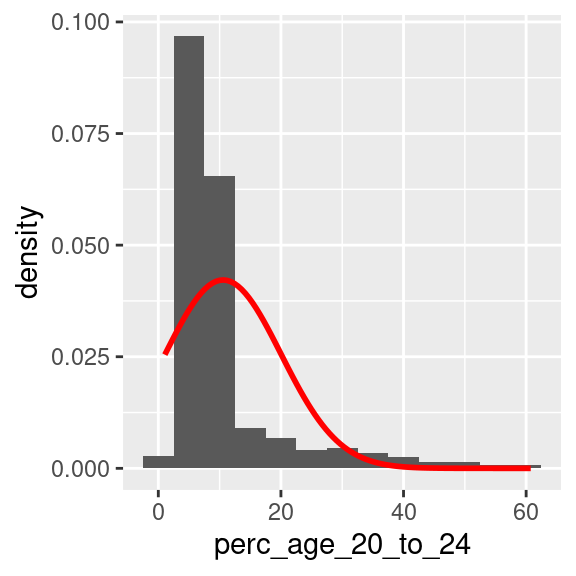
As perc_age_20_to_24 is a heavy-tailed distribution, skewed towards low values, it is not surprising that the normtest.p value indicates that the Shapiro–Wilk test is significant, which indicates that the distribution is not normal.

The code below present the output of the shapiro.test function, which only present the outcome of a Shapiro–Wilk test on the values provided as input. The output values are the same as the values reported by the norm section of stat.desc. Note that the shapiro.test function require the argument to be a numeric vector. Thus the pull function must be used to extract the perc_age_20_to_24 column from leic_2011OAC_20to24 as a vector, whereas using select with a single column name as the argument would produce as output a table with a single column.

leic_2011OAC_20to24 %>%
  pull(perc_age_20_to_24) %>%
  shapiro.test()

## 
##  Shapiro-Wilk normality test
## 
## data:  .
## W = 0.64491, p-value < 2.2e-16

As the null hypothesis of the Shapiro–Wilk test is that the sample is normally distributed, a p value lower than a 0.01 threshold (p < .01) indicates that the probability of that being true is very low. So, the flipper length of penguins in the Palmer Station dataset is not normally distributed.

The two code snippets below can be used to visualise a density-based histogram including the shape of a normal distribution having the same mean and standard deviation, and a Q-Q plot, to visually confirm the fact that perc_age_20_to_24 is not normally distributed.

leic_2011OAC_20to24 %>%
  ggplot(
    aes(
      x = perc_age_20_to_24
    )
  ) +
  geom_histogram(
    aes(
      y =..density..
    ),
    binwidth = 5
  ) + 
  stat_function(
    fun = dnorm, 
    args = list(
      mean = leic_2011OAC_20to24 %>% pull(perc_age_20_to_24) %>% mean(),
      sd = leic_2011OAC_20to24 %>% pull(perc_age_20_to_24) %>% sd()
    ),
    colour = "red", size = 1
  )

A Q-Q plot in R can be created using a variety of functions. In the example below, the plot is created using the stat_qq and stat_qq_line functions of the ggplot2 library. Note that the perc_age_20_to_24 variable is mapped to a particular option of aes that is sample.

If perc_age_20_to_24 had been normally distributed, the dots in the Q-Q plot would be distributed straight on the line included in the plot.

leic_2011OAC_20to24 %>%
  ggplot(
    aes(
      sample = perc_age_20_to_24
    )
  ) +
  stat_qq() +
  stat_qq_line()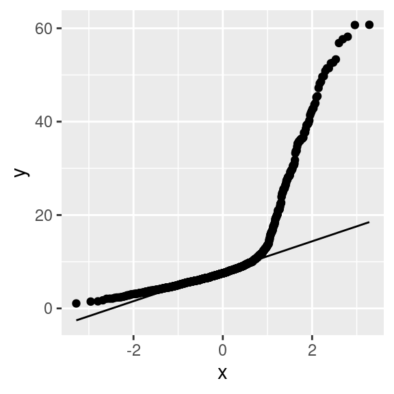

6.4 Exercise 202.1

Create a new RMarkdown document, and add the code necessary to recreate the table leic_2011OAC_20to24 used in the example above. Use the code below to re-shape the table leic_2011OAC_20to24 by pivoting the perc_age_20_to_24 column wider into multiple columns using supgrpname as new column names.

leic_2011OAC_20to24_supgrp <- leic_2011OAC_20to24 %>%
  pivot_wider(
    names_from = supgrpname,
    values_from = perc_age_20_to_24
  )

That manipulation creates one column per supergroup, containing the perc_age_20_to_24 if the OA is part of that supergroup, or an NA value if the OA is not part of the supergroup. The transformation is illustrated in the two tables below. The first shows an extract from the original leic_2011OAC_20to24 dataset, followed by the wide version leic_2011OAC_20to24_supgrp.

leic_2011OAC_20to24 %>%
  slice_min(OA11CD, n = 10) %>%
  kable(digits = 3)

OA11CD	supgrpname	perc_age_20_to_24
E00068657	HP	6.053
E00068658	MM	6.964
E00068659	MM	8.383
E00068660	MM	4.643
E00068661	MM	10.625
E00068662	MM	8.284
E00068663	MM	8.357
E00068664	MM	3.597
E00068665	MM	7.068
E00068666	MM	5.864

leic_2011OAC_20to24_supgrp %>%
  slice_min(OA11CD, n = 10) %>%
  kable(digits = 3)

OA11CD	SU	CP	MM	EC	CD	HP	UR
E00068657	NA	NA	NA	NA	NA	6.053	NA
E00068658	NA	NA	6.964	NA	NA	NA	NA
E00068659	NA	NA	8.383	NA	NA	NA	NA
E00068660	NA	NA	4.643	NA	NA	NA	NA
E00068661	NA	NA	10.625	NA	NA	NA	NA
E00068662	NA	NA	8.284	NA	NA	NA	NA
E00068663	NA	NA	8.357	NA	NA	NA	NA
E00068664	NA	NA	3.597	NA	NA	NA	NA
E00068665	NA	NA	7.068	NA	NA	NA	NA
E00068666	NA	NA	5.864	NA	NA	NA	NA

Question 202.1.1: The code below uses the newly created leic_2011OAC_20to24_supgrp table to calculate the descriptive statistics calculated for the variable leic_2011OAC_20to24 for each supergroup. Is leic_2011OAC_20to24 normally distributed in any of the subgroups? If yes, which supergroups and based on which values do you justify that claim? (Write up to 200 words)

leic_2011OAC_20to24_supgrp %>%
  select(-OA11CD) %>%
  stat.desc(norm = TRUE) %>%
  kable(digits = 3)

	SU	CP	MM	EC	CD	HP	UR
nbr.val	54.000	83.000	573.000	57.000	36.000	101.000	65.000
nbr.null	0.000	0.000	0.000	0.000	0.000	0.000	0.000
nbr.na	915.000	886.000	396.000	912.000	933.000	868.000	904.000
min	1.462	3.141	2.490	2.066	1.064	1.515	2.256
max	9.562	60.751	52.507	36.299	12.963	11.261	13.505
range	8.100	57.609	50.018	34.233	11.899	9.746	11.249
sum	295.867	2646.551	5214.286	838.415	252.108	619.266	372.010
median	5.476	30.457	7.880	10.881	6.854	6.053	5.380
mean	5.479	31.886	9.100	14.709	7.003	6.131	5.723
SE.mean	0.233	1.574	0.230	1.373	0.471	0.172	0.264
CI.mean.0.95	0.467	3.131	0.452	2.751	0.956	0.341	0.528
var	2.929	205.556	30.285	107.523	7.983	2.980	4.545
std.dev	1.712	14.337	5.503	10.369	2.825	1.726	2.132
coef.var	0.312	0.450	0.605	0.705	0.403	0.282	0.372
skewness	0.005	0.067	3.320	0.633	0.322	0.124	1.042
skew.2SE	0.008	0.127	16.266	1.001	0.410	0.258	1.753
kurtosis	-0.391	-0.825	15.143	-1.009	-0.142	0.220	1.441
kurt.2SE	-0.306	-0.789	37.156	-0.810	-0.093	0.231	1.229
normtest.W	0.991	0.980	0.684	0.889	0.965	0.993	0.937
normtest.p	0.954	0.239	0.000	0.000	0.310	0.886	0.002

Question 202.1.2: Write the code necessary to test again the normality of leic_2011OAC_20to24 for the supergroups where the analysis conducted for Question 202.1.1 indicated they are normal, using the function shapiro.test, and draw the respective Q-Q plot.

Question 202.1.3: Observe the output of the Levene’s test executed below. What does the result tell you about the variance of perc_age_20_to_24 in supergroups?

Note that the leveneTest was not designed to work with a Tidyverse approach. As such, the code below uses the . argument placeholder to specify that the input table leic_2011OAC_20to24 which is coming down from the pipe should be used as argument for the data parameter.

leic_2011OAC_20to24 %>% 
  leveneTest(
    perc_age_20_to_24 ~ supgrpname, 
    data = .
  )

## Levene's Test for Homogeneity of Variance (center = median)
##        Df F value    Pr(>F)    
## group   6  62.011 < 2.2e-16 ***
##       962                      
## ---
## Signif. codes:  0 '***' 0.001 '**' 0.01 '*' 0.05 '.' 0.1 ' ' 1

by Stefano De Sabbata – text licensed under the CC BY-SA 4.0, contains public sector information licensed under the Open Government Licence v3.0, code licensed under the GNU GPL v3.0.

5 Exploratory visualisation

7 Comparing data