2 Reproducible data science

Print this chapter

2.1 Data science

Singleton and Arribas-Bel define “geographic data science” as a space that “effectively combines the long-standing tradition and epistemologies of Geographic Information Science and Geography with many of the recent advances that have given Data Science its relevance in an emerging ‘datafied’ world” (Singleton and Arribas-Bel, 2021, p67⁹). In particular, they argue that “data science” emerged as a term to indicate the use of statistical and visual analytics tool to study a world where the digitalisation of everyday life resulted in a “data deluge” commonly referred to as “big data”¹⁰. The academic debate about the historical and epistemological background of the term “data science” is quite complex, but the term has now acquired wide-spread usage.

As such, “data science” is commonly used to refer to a set of tools and approaches to analysing data, including statistical analysis, visualisation and (what used to be referred to as) data mining. Data science also overlaps with the field of machine learning, which is a part of artificial intelligence and includes methods normally under the umbrella of statistics. If, at this point, you are confused, don’t worry, that’s quite normal. These definitions are frequently debated and frequently prone to become buzzwords.

This book focuses on an introduction to data science using R and a focus on geographic themes, although not necessarily using spatial analysis (i.e., when spatial relationships are part of the computation), which is covered in another module and wonderful books such as An Introduction to R for Spatial Analysis and Mapping by Chris Brunsdon and Lex Comber and Geocomputation with R by Robin Lovelace, Jakub Nowosad and Jannes Muenchow.

2.2 Reproducibility

According to Christopher Gandrud¹¹, a quantitative analysis or project can be considered to be reproducible if: “the data and code used to make a finding are available and they are sufficient for an independent researcher to recreate the finding”. Reproducibility practices are rooted in software engineering, including project design practices (such as Scrum), software readability principles, testing and versioning.

In GIScience, programming was essential to interact with early GIS software such as ArcInfo in the 1980s and 1990s, up until the release of the ArcGIS 8.0 suite in 1999, which included a graphical user interface. The past decade has seen a gradual return to programming and scripting in GIS, especially where languages such as R and Python allowed to combine GIS capabilities with much broader data science and machine learning functionalities. Many disciplines have seen a similar trajectory, and as programming and data science become more integral to science, reproducibility practices become a cornerstone of scientific development.

Nowadays, many academic journals and conferences require some level of reproducibility when submitting a paper (e.g., see the AGILE Reproducible Paper Guidelines from the Association of Geographic Information Laboratories in Europe). Companies are keen on reproducible analysis, which is more reliable and more efficient in the long term. Second, as the amount of data increases, reproducible approaches effectively create reliable analyses that can be more easily verified and reproduced on different or new data. Alex David Singleton, Seth Spielman, and Chris Brunsdon¹² have discussed the issue of reproducibility in GIScience, identifying the following best practices:

1. “Data should be accessible within the public domain and available to researchers”.
2. “Software used should have open code and be scrutable”.
3. “Workflows should be public and link data, software, methods of analysis and presentation with discursive narrative”.
4. “The peer review process and academic publishing should require submission of a workflow model and ideally open archiving of those materials necessary for replication”.
5. “Where full reproducibility is not possible (commercial software or sensitive data) aim to adopt aspects attainable within circumstances”.

The rest of the chapter discusses three tools that can help you improve the reproducibility of your code: Markdown, RMarkdown and Git.

2.3 R Projects

RStudio provides an extremely useful functionality to organise all your code and data, that is R Projects. Those are specialised files that RStudio can use to store all the information it has on a specific project that you are working on – Environment, History, working directory, and much more, as we will see in the coming weeks. Working with well-organised project is crucial in reproducible data science.

In RStudio Server, in the Files tab of the bottom-left panel, click on Home to make sure you are in your home folder – if you are working on your own computer, create a folder for these practicals wherever most convenient. Click on New Folder and enter Practicals in the prompt dialogue to create a folder named Practicals.

Select File > New Project … from the main menu, then from the prompt menu, New Directory, and then New Project. Insert GY7702-practical-102 as the directory name, and select the Practicals folder for the field Create project as subdirectory of. Finally, click Create Project.

RStudio has now created the project, and it should have activated it. If that is the case, the Files tab in the bottom-right panel should be in the GY7702-practical-102 folder, which contains only the GY7702-practical-102.Rproj file. The GY7702-practical-102.Rproj stores all the Environment information for the current project, and all the project files (e.g., R scripts, data, output files) should be stored within the GY7702-practical-102 folder. Moreover, the GY7702-practical-102 is now your working directory, which means that you can refer to a file in the folder by using only its name and if you save a file, that is the default directory where to save it.

On the top-right corner of RStudio, you should see a blue icon representing an R in a cube next to the name of the project (GY7702-practical-102). That also indicates that you are within the GY7702-practical-102 project. Click on GY7702-practical-102 and select Close Project to close the project. Next to the R in a cube icon, you should now see Project: (None). Click on Project: (None) and select GY7702-practical-102 from the list to reactivate the GY7702-practical-102 project. In the future, you will thus be able to close and reactivate this or any other project as necessary, depending on what you are working with. Projects can also be activated by clicking on the related .Rproj file in the Files tab in the bottom-right panel or through the Open Project… option in the file menu.

With the GY7702-practical-102 project activated, select from the top menu File > New File > RMarkdown to create a new RMarkdown document – you can use the default options in the creation menu, as this is just an example. Save and knit the RMarkdown document (as shown in the previous chapter). As you can see, both the RMarkdown file and the knitted are saved within the GY7702-practical-102 folder.

2.4 R Scripts

The RStudio Console is handy to interacting with the R interpreter and obtain results of operations and commands. However, moving from simple instructions to an actual program or script to conduct data analysis, the Console is usually not sufficient anymore. In fact, the Console is not a very comfortable way of providing long and complex instructions to the interpreter. For instance, it doesn’t easily allow you to overwrite past instructions when you want to change something in your procedure. A better option to create programs or data analysis scripts of any significant size is to use the RStudio integrated editor to create an R script.

To create an R script, select from the top menu File > New File > R Script. That opens the embedded RStudio editor and a new empty R script folder. Copy the two lines below into the file. The first loads the tidyverse library, whereas the second simply calculates the square root of two.

# Load the Tidyverse
library(tidyverse)

# Calculate the square root of two
2 %>% sqrt()

## [1] 1.414214

As you can see, a comment precedes each line, describing what the subsequent command does. Adequately commenting the code is a fundamental practice in programming. As this is a learning resource, the comments in the examples below explain “what” the subsequent lines of code do. However, comments should generally focus on “how” a procedure (i.e., an algorithm) is implemented in a set of instructions (i.e., a section of the script) and crucially on “why” the procedure has been implemented in a specific way. We will see more complex examples in the rest of this book.

From the top menu, select File > Save, type in my-first-script.R (make sure to include the underscore and the .R extension) as File name, and click Save. Finally, click the Source button on the top-right of the editor.

Congratulations, you have executed your first R script! 😊👍

You can then edit the script by adding (for instance) the new lines of code shown below, saving the file, and executing the script’s new version. RStudio also allows to select one or more lines and click Run to execute only the selected lines or the line where the cursor currently is.

# First variable in a script:
# the line below uses the Sys.time of the base library 
# to obtain the current time as a character string
current_time <- Sys.time()
print(current_time)

Self-test questions:

• What happens if you select print(current_time) and click Run to run just that line?
• What happens if you click the Source button again and thus execute the new version of the script?
• What happens if you click the Source a third time?
• How do the three differ (if they do)?

2.4.1 Reproducible workflows

The readr library (also part of the Tidyverse) provides a series of functions that can be used to load from and save data to different file formats. The read_csv function reads a Comma Separated Values (CSV) file from the path provided as the first argument.

The code below loads the 2011_OAC_Raw_uVariables_Leicester.csv containing the 2011 Output Area Classification (2011 OAC) for Leicester. The 2011 OAC is a geodemographic classification of the census Output Areas (OA) of the UK, which was created by Gale et al. (2016) starting from an initial set of 167 prospective variables from the United Kingdom Census 2011: 86 were removed, 41 were retained as they are, and 40 were combined, leading to a final set of 60 variables. Gale et al. (2016) finally used the k-means clustering approach to create 8 clusters or supergroups (see map at datashine.org.uk), as well as 26 groups and 76 subgroups. The dataset in the file 2011_OAC_Raw_uVariables_Leicester.csv contains all the original 167 variables, as well as the resulting groups, for the city of Leicester. The full variable names can be found in the file 2011_OAC_Raw_uVariables_Lookup.csv.

The read_csv instruction throws a warning that shows the assumptions about the data types used when loading the data. As illustrated by the output of the last line of code, the data are loaded as a tibble 969 x 190, that is 969 rows – one for each OA – and 190 columns, 167 of which represent the input variables used to create the 2011 OAC. The function write_csv can similarly be used to save a dataset as a csv file, as illustrated in the exercise below.

library(tidyverse)
library(knitr)

# Read the Leicester 2011 OAC dataset from the csv file
leicester_2011OAC <- 
  read_csv("2011_OAC_Raw_uVariables_Leicester.csv")

OA11CD	LSOA11CD	supgrpcode	supgrpname	Total_Population
E00069517	E01013785	6	Suburbanites	313
E00069514	E01013784	2	Cosmopolitans	323
E00169516	E01013713	4	Multicultural Metropolitans	341

Both read_csv and write_csv require to specify a file path, that can be specified in two different ways:

• Absolute file path: the full file path from the root folder of your computer to the file.
  • The absolute file path of a file can be obtained using the file.choose() instruction from the R Console, which will open an interactive window that will allow you to select a file from your computer. The absolute path to that file will be printed to the console.
  • Absolute file paths provide a direct link to a specific file and ensure that you are loading that exact file.
  • However, absolute file paths can be problematic if the file is moved or if the script is run on a different system, and the file path would then be invalid
• Relative file path: a partial path from the current working folder to the file.
  • The current working directory (current folder) is part of the environment of the R session and can be identified using the getwd() instruction from the `R Console*.
    • When a new R session is started, the current working directory is usually the computer user’s home folder.
    • When working within an R project, the current working directory is the project directory.
    • The current working can be manually set to a specific directory using the function setwd.
  • Using a relative path while working within an R project is the option that provides the best overall consistency, assuming that all (data) files to be read by scripts of a project are also contained in the project folder (or subfolder).

# Absolute file path
# Note: the first / indicates the root folder
read_csv("/home/username/GY7702/data/2011_OAC_Raw_uVariables_Leicester.csv")

# Relative file path
# assuming the working directory is the user's home folder
# /home/username
# Note: no initial / for relative file paths
read_csv("GY7702/data/2011_OAC_Raw_uVariables_Leicester.csv")


# Relative file path
# assuming you are working within an R project created in the folder
# /home/username/GY7702
# Note: no initial / for relative file paths
read_csv("data/2011_OAC_Raw_uVariables_Leicester.csv")

2.4.2 Exercise 102.1

Create a new subfolder named data within the R project GY7702-practical-102 and upload the 2011_OAC_Raw_uVariables_Leicester.csv file into the data folder¹³.

Create a new R script named students-around-campus.R including the reproducible workflow defined in the code below, which uses the tidyverse functions read_csv and write_csv, as well as the select and filter functions – will be discussed in detail in the next chapter, don’t worry too much about them for now 😊 – to execute the following steps:

1. read the 2011 OAC file 2011_OAC_Raw_uVariables_Leicester.csv directly from the file, but without storing it into a variable;
2. select the OA codes variable, and the variables representing the code and name of the supergroup and group assigned to each OA by the 2011 OAC (supgrpcode and supgrpname, as well as grpcode and grpname);
3. filter only the OAs classified as part of the Students Around Campus group in the 2011 OAC;
4. write the results to a file named 2011_OAC_Leicester_StudentsAroundCampus.csv, which is your own version of the 2011_OAC_supgrp_Leicester.csv.

Save and run the script. The new dataset written into a csv file can then be loaded into any other software, such as a GIS, to further analyse or visualise the data. At the same time, R offers a wide range of tools to both analyse or visualise, as we will see in this and other modules. You can download and inspect the file to verify that only contains seven columns mentioned in the code, and that all rows have "Students Around Campus" as value for the column grpname.

read_csv("data/2011_OAC_Raw_uVariables_Leicester.csv") %>%
  select(
    OA11CD, LSOA11CD, 
    supgrpcode, supgrpname,
    grpcode, grpname,
    Total_Population
  ) %>%
  filter(grpname == "Students Around Campus") %>%
  write_csv("data/2011_OAC_Leicester_StudentsAroundCampus.csv")

2.5 RMarkdown

An essential tool used in creating this book is RMarkdown, an R library that allows you to create scripts that mix the Markdown mark-up language and R, to create dynamic documents. RMarkdown script can be compiled, at which point the Markdown notation is interpreted to create the output files, while the R code is executed and the output incorporated in the document.

For instance, the following markdown code

[This is a link to the University of Leicester](http://le.ac.uk) and **this is in bold**.

is rendered as

This is a link to the University of Leicester and this is in bold.

The core Markdown notation used in this chapter is presented below. A full RMarkdown cheatsheet is available here.

# Header 1
## Header 2
### Header 3
#### Header 4
##### Header 5

**bold**
*italics*

[This is a link to the University of Leicester](http://le.ac.uk)

- Example list
    - Main folder
        - Analysis
        - Data
        - Utils
    - Other bullet point
- And so on
    - and so forth

1. These are
    1. Numeric bullet points
    2. Number two
2. Another number two
3. This is number three

R code can be embedded in RMarkdown documents using code snippets, as in the example below. That results in the code chunk being displayed within the document (as echo=TRUE is specified), followed by the output from the execution of the same code.

```{r, echo=TRUE}
a_number <- 0
a_number <- a_number + 1
a_number <- a_number + 1
a_number <- a_number + 1
a_number
```

a_number <- 0
a_number <- a_number + 1
a_number <- a_number + 1
a_number <- a_number + 1
a_number

## [1] 3

To create an RMarkdown document in RStudio, select File > New File > R Markdown … – this might prompt RStudio to update some packages. Once the RMarkdown document creation menu appears, specify “Practical 102” as the title and your name as the author, and select PDF as the output format. The new document should contain the core document information, plus some additional content that simply explains how RMarkdown works.

Read the document through, inspecting both the R and the Markdown code. Note how the information provided in the previous step is encoded in the first five lines which compose the heading. For each code snippet, the option echo=TRUE tells RStudio to include the code in the output document, along with the output of the computation. If echo=FALSE is specified, the code will be omitted. If the option message=FALSE and warning=FALSE are added, messages and warnings from R are not displayed in the output document.

Save the document (File > Save) as my-first-rmarkdown.Rmd and then click the Knit button visible above the file panel in RStudio to compile the source file into a PDF file – if the browser blocks the opening for the new file in a window, please allow the pop-up to open from the top-right of your browser. Read through the compiled document and compare it to the source document to assess how the compiled document is derived from the source.

2.5.1 Exercise 102.2

Create a new RMarkdown document using Students around campus in Leicester as the title and PDF as the output file type. Delete the example code and add the code below, which includes a markdown second-heading section named Libraries and a chunk loading the tidyverse and knitr libraries. Save the file with the name students-around-campus-map.Rmd in the Leicester_population project.

---
title: "Students around campus in Leicester"
output: pdf_document
date: "2022-10-20"
---

```{r setup, include=FALSE}
knitr::opts_chunk$set(echo = TRUE)
```

## Libraries

```{r libraries, warning=FALSE, message=FALSE}
library(tidyverse)
library(knitr)
```

Upload the Leicester_2011_OAs.geojson to the data folder, then add a new markdown second-heading section named Map and a new R chunk. In the new R chunk, copy-paste the code below which uses a range of functions that we will see in the coming weeks, alongside the sf and mapsf libraries, to create a map showing the location of the OAs classified as part of the Students Around Campus group in the 2011 OAC.

Again, as mentioned above, don’t worry too much about the details of the code right now. We will get to those in the coming weeks. Focus on understanding and embracing the reproducible data science workflow. 😊

library(tidyverse)
library(sf)
library(mapsf)

leicester_2011OAC_students <- 
  read_csv("data/2011_OAC_Raw_uVariables_Leicester.csv") %>%
      filter(grpname == "Students Around Campus")

st_read("data/Leicester_2011_OAs.geojson") %>%
  left_join(leicester_2011OAC_students) %>% 
  mf_map(
    var = "grpname", 
    type = "typo",
    pal = "Dark 3",
    leg_title = "2011 OAC groups",
    leg_no_data = "Other groups"
    )
mf_credits(txt = "Source: Office for National Statistics, Census 2021. Contains National Statistics data Crown copyright and database right 2022; Contains Ordnance Survey data Crown copyright and database right 2022.")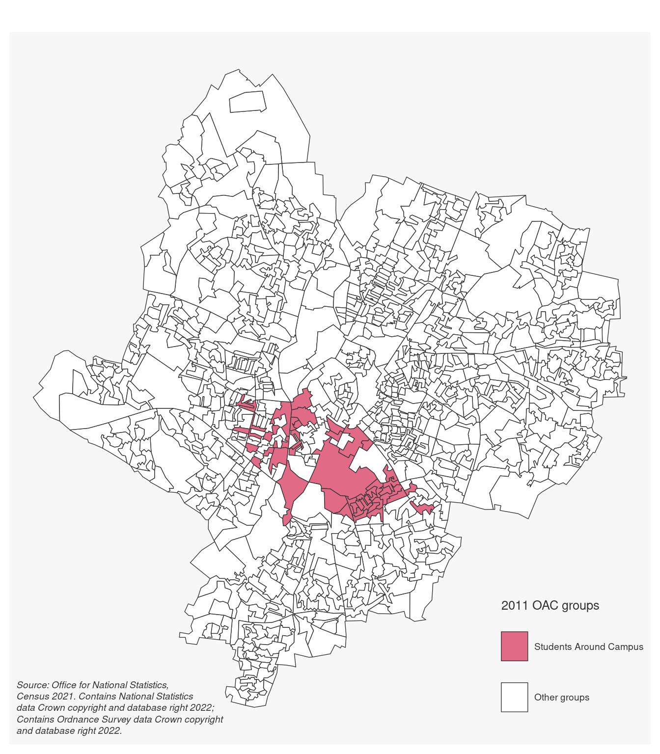

2.6 How to cite

2.6.1 References

Academic references can be added to RMarkdown as illustrated in the R Markdown Cookbook.¹⁴ Bibtex references can be added to a separate .bib file that is linked to in the heading of the RMarkdown document. References can then be cited using the @ symbol followed by the reference id.

For instance, this documents links to the references.bib bibtex file, which contains the academic references, and the packages.bib bibtex files, which contains additional references for the R packages (see also next section), by adding the following line in the heading.

bibliography: [references.bib, packages.bib]

The references.bib contains the following reference for the R Markdown Cookbook book.

@book{xie2020r,
  title={R markdown cookbook},
  author={Xie, Yihui and Dervieux, Christophe and Riederer, Emily},
  year={2020},
  publisher={Chapman and Hall/CRC},
  url = {https://bookdown.org/yihui/rmarkdown-cookbook/}
}

That allows writing the first sentence of this section as follows.

Academic references can be added to RMarkdown [as illustrated in the R Markdown Cookbook](https://bookdown.org/yihui/rmarkdown-cookbook/bibliography.html) [@xie2020r].

Bibtex references can be obtained from most journals or by clicking on the Cite link under a paper in Google Scholar and then selecting Bibtex.

2.6.2 Code

The UK’s Software Sustainability Institute provides clear guidance about how to cite software written by others. As outlined in the guidance, you should always cite and credit their work. However, using academic-style citations is not always straightforward when working with libraries, as most of them are not linked to an academic paper nor provide a DOI. In such cases, you should at least include a link to the authors’ website or repository in the script or final report when using a library. For instance, you can add a link to the Tidyverse’s website, repository or CRAN page when using the library. However, Wickham et al.¹⁵ also wrote a paper on their work on the Tidyverse for the Journal of Open Source Software, so you can also cite their paper using Bibtex in RMarkdown.

Appropriate citations are even more important when directly copying or adapting code from others’ work. Plagiarism principles apply to code as much as they do to text. The Massachusetts Institute of Technology (MIT)’s Academic Integrity at MIT: A Handbook for Students includes a section on writing code which provides good guidance on when and how to cite code that you include in your projects or you adapt for your own code properly. That also applies to re-using your own code, which you have written before. It is important that you refer to your previous work and fully acknowledge all previous work that has been used in a project so that others can find everything you have used in a project.

It is common practice to follow a particular referencing style for the in-text quotations, references and bibliography, such as the Harvard style (see, e.g., the Harvard Format Citation Guide available Mendeley’s help pages). Following such guidelines will not only ensure that others can more easily use and reproduce your work but also that you demonstrate academic honesty and integrity.

---

by Stefano De Sabbata – text licensed under the CC BY-SA 4.0, contains public sector information licensed under the Open Government Licence v3.0, code licensed under the GNU GPL v3.0.