9 Multiple regression
This chapter focuses on regression analysis, starting from simple regression and then multiple regression analysis. Both sections discuss how to run a regression analysis and (importantly) how to check that the analysis meets the test assumptions and how to report the results in an analysis document.
The multiple regression analysis is a supervised machine learning approach to creating a model able to predict the value of one outcome variable \(Y\) based on two or more predictor variables \(X_1 \dots X_M\), by estimating the intercept \(b_0\) and the coefficients (slopes) \(b_1 \dots b_M\), and accounting for a reasonable amount of error \(\epsilon\).
\[Y_i = (b_0 + b_1 * X_{i1} + b_2 * X_{i2} + \dots + b_M * X_{iM}) + \epsilon_i \]
The assumptions are the same as the simple regression, plus the assumption of no multicollinearity: if two or more predictor variables are used in the model, each pair of variables not correlated. This assumption can be tested by checking the variance inflation factor (VIF). If the largest VIF value is greater than 10 or the average VIF is substantially greater than 1, there might be an issue of multicollinearity.
9.0.1 Multiple regression example
The example below explores whether a regression model can be created to estimate the number of people in Leicester commuting to work using private transport (u121 in the 2011 Output Area Classification dataset seen in previous chapters) in Leicester, using the number of people in different industry sectors as predictors.
For instance, occupations such as electricity, gas, steam and air conditioning supply (u144) require to travel some distances with equipment, thus the related variable u144 is included in the model, whereas people working in information and communication might be more likely to work from home or commute by public transport.
leicester_2011OAC <- read_csv("2011_OAC_Raw_uVariables_Leicester.csv")
# Select and
# normalise variables
leicester_2011OAC_transp <-
  leicester_2011OAC %>%
  select(
    OA11CD,
    Total_Pop_No_NI_Students_16_to_74, Total_Employment_16_to_74,
    u121, u141:u158
  ) %>%
  # percentage method of travel
  mutate(
    u121 = (u121 / Total_Pop_No_NI_Students_16_to_74) * 100
  ) %>%
  # percentage across industry sector columns
  mutate(
    across(
      u141:u158,
      function(x){ (x / Total_Employment_16_to_74) * 100 }
    )
  ) %>%
  # rename columns
  rename_with(
    function(x){ paste0("perc_", x) },
    c(u121, u141:u158)
  ) %>%
  arrange(perc_u121)
Let’s observe how all those variable relate to one another using a pairs plot.
library(GGally)

leicester_2011OAC_transp %>%
  select(perc_u121, perc_u141:perc_u158) %>%
  ggpairs(
    upper = list(continuous =
        wrap(ggally_cor, method = "kendall")),
    lower = list(continuous =
        wrap("points", alpha = 0.3, size=0.1))
  ) +
  theme_bw()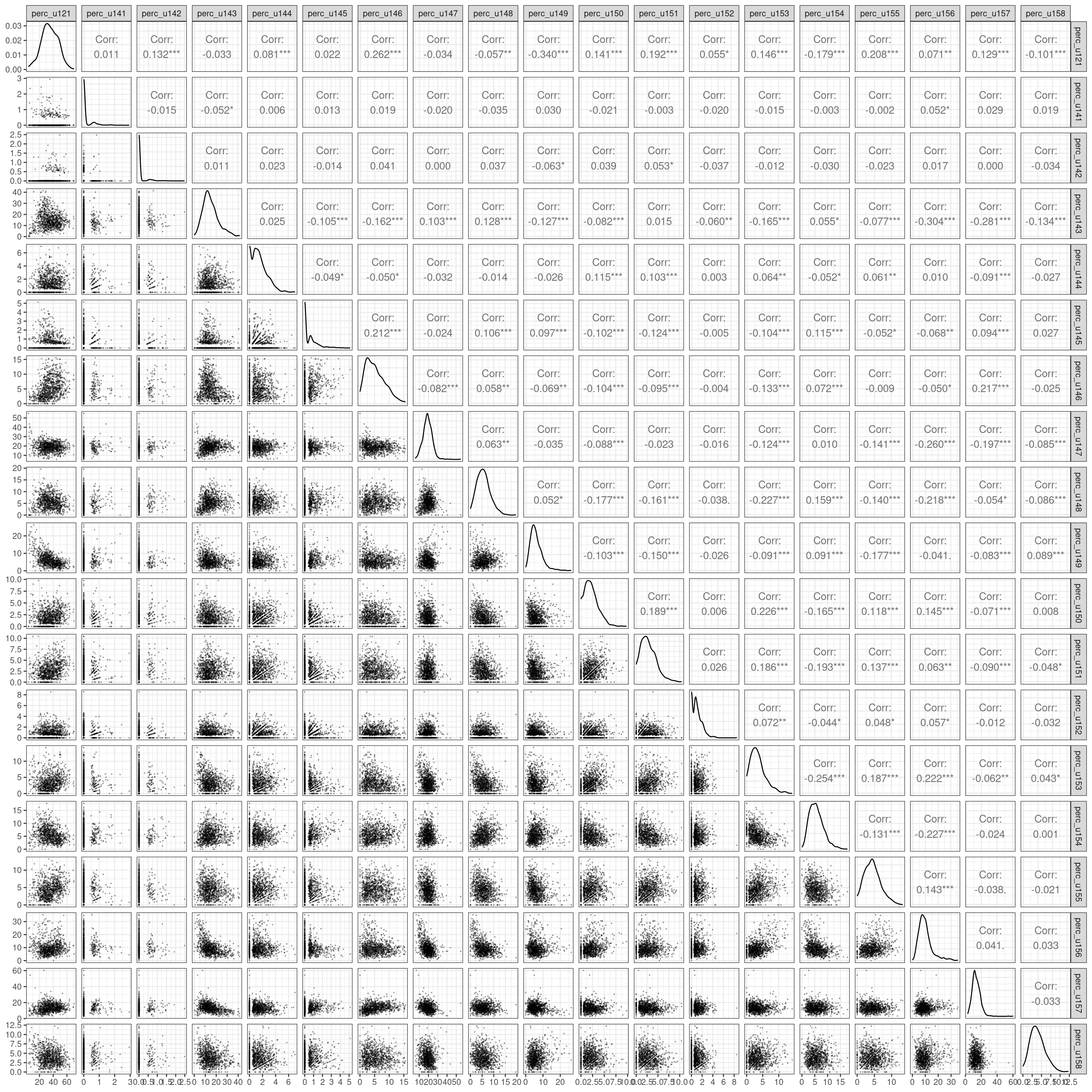
Based on the plot above and our understanding of the variables, we can try create a model able to relate and estimate the dependent (output) variable perc_u120 (Method of Travel to Work, Private Transport) with the independent (predictor) variables:
-
perc_u142: Industry Sector, Mining and quarrying -
perc_u144: Industry Sector, Electricity, gas, steam and air conditioning … -
perc_u146: Industry Sector, Construction -
perc_u149: Industry Sector, Accommodation and food service activities
A multiple regression model can be specified in a similar way as a simple regression model, using the same lm function, but adding the additional predictor variables using a + operator.
# Create model
commuting_model1 <-
  leicester_2011OAC_transp %$%
  lm(
    perc_u121 ~
      perc_u142 + perc_u144 + perc_u146 + perc_u149
  )

# Print summary
commuting_model1 %>%
  summary()
##
## Call:
## lm(formula = perc_u121 ~ perc_u142 + perc_u144 + perc_u146 +
## perc_u149)
##
## Residuals:
## Min 1Q Median 3Q Max
## -35.315 -6.598 -0.244 6.439 31.472
##
## Coefficients:
## Estimate Std. Error t value Pr(>|t|)
## (Intercept) 37.12690 0.94148 39.434 < 2e-16 ***
## perc_u142 3.74768 1.21255 3.091 0.00205 **
## perc_u144 1.16865 0.25328 4.614 4.48e-06 ***
## perc_u146 1.05408 0.09335 11.291 < 2e-16 ***
## perc_u149 -1.56948 0.08435 -18.606 < 2e-16 ***
## ---
## Signif. codes: 0 '***' 0.001 '**' 0.01 '*' 0.05 '.' 0.1 ' ' 1
##
## Residual standard error: 9.481 on 964 degrees of freedom
## Multiple R-squared: 0.3846, Adjusted R-squared: 0.3821
## F-statistic: 150.6 on 4 and 964 DF, p-value: < 2.2e-16
# Not rendered in bookdown
stargazer(commuting_model1, header=FALSE)
commuting_model1 %>%
  rstandard() %>%
  shapiro.test()
##
## Shapiro-Wilk normality test
##
## data: .
## W = 0.99889, p-value = 0.8307##
## studentized Breusch-Pagan test
##
## data: .
## BP = 28.403, df = 4, p-value = 1.033e-05##
## Durbin-Watson test
##
## data: .
## DW = 0.72548, p-value < 2.2e-16
## alternative hypothesis: true autocorrelation is greater than 0## perc_u142 perc_u144 perc_u146 perc_u149
## 1.006906 1.016578 1.037422 1.035663The output above suggests that the model is fit (\(F(4, 964) = 150.62\), \(p < .001\)), indicating that a model based on the presence of people working in the four selected industry sectors can account for 38.21% of the number of people using private transportation to commute to work. However the model is only partially robust. The residuals are normally distributed (Shapiro-Wilk test, \(W = 1\), \(p =0.83\)) and there seems to be no multicollinearity with average VIF \(1.02\), but the residuals don’t satisfy the homoscedasticity assumption (Breusch-Pagan test, \(BP = 28.4\), \(p < .001\)), nor the independence assumption (Durbin-Watson test, \(DW = 0.73\), \(p < .01\)).
The coefficient values calculated by the lm functions are important to create the model, and provide useful information. For instance, the coefficient for the variable perc_u144 is 1.169, which indicates that if the presence of people working in electricity, gas, steam and air conditioning supply increases by one percentage point, the number of people using private transportation to commute to work increases by 1.169 percentage points, according to the model. The coefficients also indicate that the presence of people working in accommodation and food service activities actually has a negative impact (in the context of the variables selected for the model) on the number of people using private transportation to commute to work.
In this example, all variables use the same unit and are of a similar type, which makes interpreting the model relatively simple. When that is not the case, it can be useful to look at the standardized \(\beta\), which provide the same information but measured in terms of standard deviation, which make comparisons between variables of different types easier to draw. For instance, the values calculated below using the function lm.beta of the library lm.beta indicate that if the presence of people working in construction has the highest impact on the outcome varaible. If the presence of people working in construction increases by one standard deviation, the number of people using private transportation to commute to work increases by 0.29 standard deviations, according to the model.
# Install lm.beta library if necessary
# install.packages("lm.beta")
library(lm.beta)

lm.beta(commuting_model1)
##
## Call:
## lm(formula = perc_u121 ~ perc_u142 + perc_u144 + perc_u146 +
## perc_u149)
##
## Standardized Coefficients::
## (Intercept) perc_u142 perc_u144 perc_u146 perc_u149
## NA 0.07836017 0.11754058 0.29057993 -0.478410839.1 Exercise 204.2
See group work exercise, Part 3.
by Stef De Sabbata – text licensed under the CC BY-SA 4.0, contains public sector information licensed under the Open Government Licence v3.0, code licensed under the GNU GPL v3.0.