1 Introduction to R

Print this chapter

We start this chapter with a brief introduction to R, the programming language that will be the focus of the module, and the tool that we will use to do data science.

R is one of the most widely used programming languages nowadays, along with Python, especially in geographic and satellite data science. I don’t personally have a strong preference for either, and I use both fairly regularly and in combination. Most of the time, using one or the other is a matter of habit or the availability of a particular functionality that makes it easier to complete the task you are set to do. For instance, Python has great libraries for programming deep neural networks. However, I find R more effective and powerful in data manipulation, statistical analysis, visualisation and mapping. That is the key reason why this book focuses on R. At the same time, beyond the mere details of syntax, the languages are not too different and are becoming easier to integrate. Most principles and approaches covered in this book can be applied when using Python, just using a different syntax.

1.1 The R programming language

R⁴ was created in 1992 by Ross Ihaka and Robert Gentleman at the University of Auckland, New Zealand. R is a free, open-source implementation of the S statistical programming language initially created at Bell Labs. At its core, R is a functional programming language (its main functionalities revolve around defining and executing functions). However, it now supports and is commonly used as an imperative (focused on instructions on variables and programming control structures) and object-oriented (involving complex object structures) programming language.

In simple terms, programming in R mainly focuses on devising a series of instructions to execute a task – most commonly, loading and analysing a dataset.

As such, R can be used to program by creating sequences of instructions involving variables – which are named entities that can store values, more on that below. That will be the main topic of this practical session. Instructions can include control flow structures, such as decision points (if/else) and loops, which will be the topic of the next practical session. Instructions can also be grouped into functions, which we will see in more detail in the next chapter.

R is interpreted, not compiled. That means that an R interpreter receives an instruction you write and interprets and executes them. Other programming languages require their code to be compiled in an executable file to be executed on a computer.

1.1.1 RStudio

RStudio is probably the most popular Integrated Development Environment (IDE) for R. When using RStudio, the R interpreter is hidden in the backend, and RStudio is the frontend application that allows you to interact with the interpreter. As you open RStudio or RStudio Server, the interface is divided into two main sections. On the left side, you find the Console – and the R script editor, when a script is being edited. The Console in an input/output window into the R interpreter, where you can type instructions and see the resulting output.

For instance, if you type in the Console

1 + 1

the R interpreter understands that as an instruction to sum 1 to 1 and returns the following result as output.

## [1] 2

As these materials are created in RMarkdown, the output of the computation is always preceded by ##. Note how the output value 2 is preceded by [1], which indicates that the output is constituted by only one element. If the output is constituted by more than one element, as the list of numbers below, each row of the output is preceded by the index of the first element of the output.

##  [1]   1   4   9  16  25  36  49  64  81 100 121 144 169 196 225 256 289 324 361
## [20] 400

On the right side, you find two groups of panels. On the top-right, the main element is the Environment panel, which represents of the current state of the interpreter’s memory, showing all the information available for computation. For instance, that is where you will be able to see datasets loaded for analysis. On the bottom-right, you find the Files panel, which shows the file system (file and folders on your computer or the server), as well as the Help panel, which shows you the help pages when required. We will discuss the other panels later on in the practical sessions.

1.1.2 Coding style

A coding style is a set of rules and guidelines to write programming code designed to ensure that the code is easy to read, understand, and consistent over time. Following a good coding style is essential when writing code that others will read – for instance, if you work in a team, publish your code or submit your code as a piece of coursework – and it ensures you will understand your code in a few months. Following a good coding style is also an essential step towards reproducibility, as we will see in a later chapter.

In this book, I will follow the Tidyverse Style Guide (style.tidyverse.org). Study the Tidyverse Style Guide and use it consistently.

1.2 Core concepts

1.2.1 Values

When a value is typed in the Console, the interpreter returns the same value. In the examples below, 2 is a simple numeric value, while "String value" is a textual value, which in R is referred to as a character value and in programming is also commonly referred to as a string (short for a string of characters).

Numeric example:

## [1] 2

Character example:

"String value"

## [1] "String value"

Note how character values need to start and end with a single or double quote (' or "), which are not part of the information themselves. The Tidyverse Style Guide suggests always using the double quote ("), so we will use those in this module.

Anything that follows a # symbol is considered a comment, and the interpreter ignores it.

# hi, I am a comment, please ignore me

As mentioned above, the interpreter understands simple operations on numeric and logic values, as well as text objects (including single characters and strings of character, that is text objects longer than one character, commonly referred to simply as strings in computer science), as discussed in more detail in Appendix 1.

# Sum 1 and 2
1 + 2

## [1] 3

# Logical AND operation between
# the value TRUE and FALSE
TRUE & FALSE

## [1] FALSE

# Check whether the character a
# is equal to the character b
"a" == "b"

## [1] FALSE

1.2.2 Variables

In computer programming, a variable can be thought about as a storage location (a bit of memory) with an associated name (also referred to as identifier) and a value that can vary – hence the name variable. When programming, you can define a variable by naming it with an identifier and providing a value to be stored in the variable. After that, you can retrieve the value stored in the variable by specifying the chosen identifier. Variables are an essential tool in programming, as they allow saving the result of a piece of computation and to retrieve it later on for further analysis.

A variable can be defined in R using an identifier (e.g., a_variable) on the left of an assignment operator <-, followed by the object to be linked to the identifier, such as a value (e.g., 1) to be assigned on the right. The value of the variable can be invoked by simply specifying the identifier.

a_variable <- 1
a_variable

## [1] 1

If you type a_variable <- 1 in the Console in RStudio, a new element appears in the Environment panel, representing the new variable in the memory. The left part of the entry contains the identifier a_variable, and the right part contains the value assigned to the variable a_variable, that is 1. In the example below, another variable named another_variable is created and summed to a_variable, saving the result in sum_of_two_variables.

another_variable <- 4
another_variable

## [1] 4

sum_of_two_variables <- a_variable + another_variable
sum_of_two_variables

## [1] 5

1.2.3 Data frames

The examples above illustrate how R allows working with simple data types. However, in data science, we rarely engage directly with such simple pieces of information. Rather, we commonly work with datasets composed of tables. Data frames are complex data types which encode the concept of a table in R by combining and arranging together a series of simple objects. In the following chapters, we will explore the different complex types and how to handle tables in more detail.

R includes many simple example data frames, such as the iris dataset. When loading R, a pre-defined variable named iris will be available in the environment. By specifying the identifier iris in the console (as shown below), you can invoke the variable and see its contents. Each one of the 150 rows of the table (the first five rows are shown below) reports information about an iris flower. Four numeric columns (Sepal.Length, Sepal.Width, Petal.Length and Petal.Width) are used to describe the size of sepal and petal, while a string column (Species) is used to catalogue the species of iris.

iris

Sepal.Length	Sepal.Width	Petal.Length	Petal.Width	Species
5.1	3.5	1.4	0.2	setosa
4.9	3.0	1.4	0.2	setosa
4.7	3.2	1.3	0.2	setosa
4.6	3.1	1.5	0.2	setosa
5.0	3.6	1.4	0.2	setosa

1.2.4 Algorithms

Any operation that can be executed using a computer is called an algorithm. To be more precise, Nigel Cutland⁵ defined an algorithm as “a mechanical rule, or automatic method, or program for performing some mathematical operation” (Cutland, 1980, p. 7⁶).

The instructions you get to mount your Ikea furniture can be thought of as an algorithm, an effective procedure to perform the operation of mounting your furniture. You are playing the part of the computer executing the algorithm.

A program is a set of instructions implementing an abstract algorithm into a specific language – let that be R, Python, or any other language. In their definition, algorithms (and thus the programs that implement them) can use variables and functions. As is the case for R, programs that are interpreted rather than compiled are also referred to as scripts.

1.2.5 Functions

You can think of a function as a processing unit that, having received some values as input, performs a specific task and can return a value as output. Some simple algorithms can be coded as programs made of only one function that performs the whole task. More complex algorithms might require multiple functions, each designed to complete a sub-task, which combined perform the entire task.

You can invoke a function by specifying the function name along with the arguments (input values) between simple brackets. Each argument corresponds to a parameter (i.e., an internal variable used within the function to run the operation, as we will see in more detail later in this book). Programming languages provide pre-defined functions that implement common algorithms (e.g., finding the square root of a number or calculating a linear regression).

For instance, sqrt is the pre-defined function in R that computes the square root of a number. The instruction sqrt(2) tells the R interpreter to run the function that calculates the square root using 2 as the input value. The function will return 1.414214, the square root of 2, as the output.

sqrt(2)

## [1] 1.414214

Another example is the function round, which returns a value rounded to a specified number of digits after the dot. For instance, round(1.414214, digits = 2) returns 1.41. In this case, we specify that the second argument refers to the number of digits to be kept, and this is because this function also has other arguments that can be specified.

round(1.414214, digits = 2)

## [1] 1.41

Functions can also be used on the right side of the assignment operator <- in which case the output value of the function will be stored in the memory slot with that identifier. Variables can be used as arguments. For instance, after saving the result of the square root of two in the variable sqrt_of_two, we can use the same variable as the first argument for the function round.

sqrt_of_two <- sqrt(2)
sqrt_of_two

## [1] 1.414214

round(sqrt_of_two, digits = 2)

## [1] 1.41

As the rest of the book will illustrate, R provides a wide range of functions that will allow conducting any step of a a data analysis: from data input/ouput to data manipulation, from statistics and machine learning to visualisation, and even to creating a web-based book like the one you are currently reading (which has indeed been created using R). For instance, you can use the function hist to plot the histogram of petal lengths of flowers in iris. Note how, in the code below, the first parameter is not iris but iris$Petal.Length as the $ is used to extract the Petal.Length from iris (more on this in the coming chapters).

hist(iris$Petal.Length, main = "Petal lengths")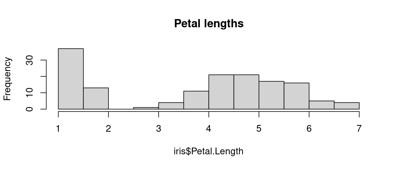

Functions can also be used as arguments of functions. Instead of first calculating the square root of two, saving the value in a variable, and then using the variable as the first argument of round, we can directly add the function sqrt and its argument as the first argument of the function round.

round(sqrt(2), digits = 2)

## [1] 1.41

In a subsequent chapter, we will see how you can create functions yourself.

As we introduce variables and functions, and functions using variables and functions, the complexity of our code increases quite rapidly. In fact, using a function as the argument for another function is usually discouraged because it makes the code more difficult to read. Instead, it would be best to always aim for a code that is as easy to read and understand as possible. An essential step in ensuring that is to follow coding style guidelines closely.

1.2.6 Libraries

Functions can be collected and stored in libraries (sometimes referred to as packages), containing related functions and sometimes datasets. For instance, the base library in R includes the sqrt function above, and the rgdal library, which contains implementations of the GDAL (Geospatial Data Abstraction Library) functionalities for R.

Libraries can be installed in R using the function install.packages or using Tool > Install Packages... in RStudio.

1.3 Tidyverse

The meta-library Tidyverse⁷ contains the following libraries:

ggplot2⁸ is a system for declaratively creating graphics based on The Grammar of Graphics. You provide the data, tell ggplot2 how to map variables to aesthetics, what graphical primitives to use, and it takes care of the details.
dplyr provides a grammar of data manipulation, providing a consistent set of verbs that solve the most common data manipulation challenges.
tidyr provides a set of functions that help you get to tidy data. Tidy data is data with a consistent form: in brief, every variable goes in a column, and every column is a variable.
readr provides a fast and friendly way to read rectangular data (like csv, tsv, and fwf). It is designed to flexibly parse many types of data found in the wild, while still cleanly failing when data unexpectedly changes.
purrr enhances R’s functional programming (FP) toolkit by providing a complete and consistent set of tools for working with functions and vectors. Once you master the basic concepts, purrr allows you to replace many for loops with code that is easier to write and more expressive.
tibble is a modern re-imagining of the data frame, keeping what time has proven to be effective, and throwing out what it has not. Tibbles are data.frames that are lazy and surly: they do less and complain more forcing you to confront problems earlier, typically leading to cleaner, more expressive code.
stringr provides a cohesive set of functions designed to make working with strings as easy as possible. It is built on top of stringi, which uses the ICU C library to provide fast, correct implementations of common string manipulations.
forcats provides a suite of useful tools that solve common problems with factors. R uses factors to handle categorical variables, variables that have a fixed and known set of possible values.

A library can be loaded using the function library, as shown below (note the name of the library is not quoted). Once a library is installed on a computer, you don’t need to install it again, but every script needs to load all the libraries that it uses. Once a library is loaded, all its functions can be used.

Important: it is always necessary to load the tidyverse meta-library if you want to use the stringr functions or the pipe operator %>%.

library(tidyverse)

1.3.1 The pipe operator

The pipe operator is useful to outline more complex operations step by step (see also R for Data Science, Chapter 18). The pipe operator %>%

takes the result from one function
and passes it to the next function
as the first argument
that doesn’t need to be included in the code anymore

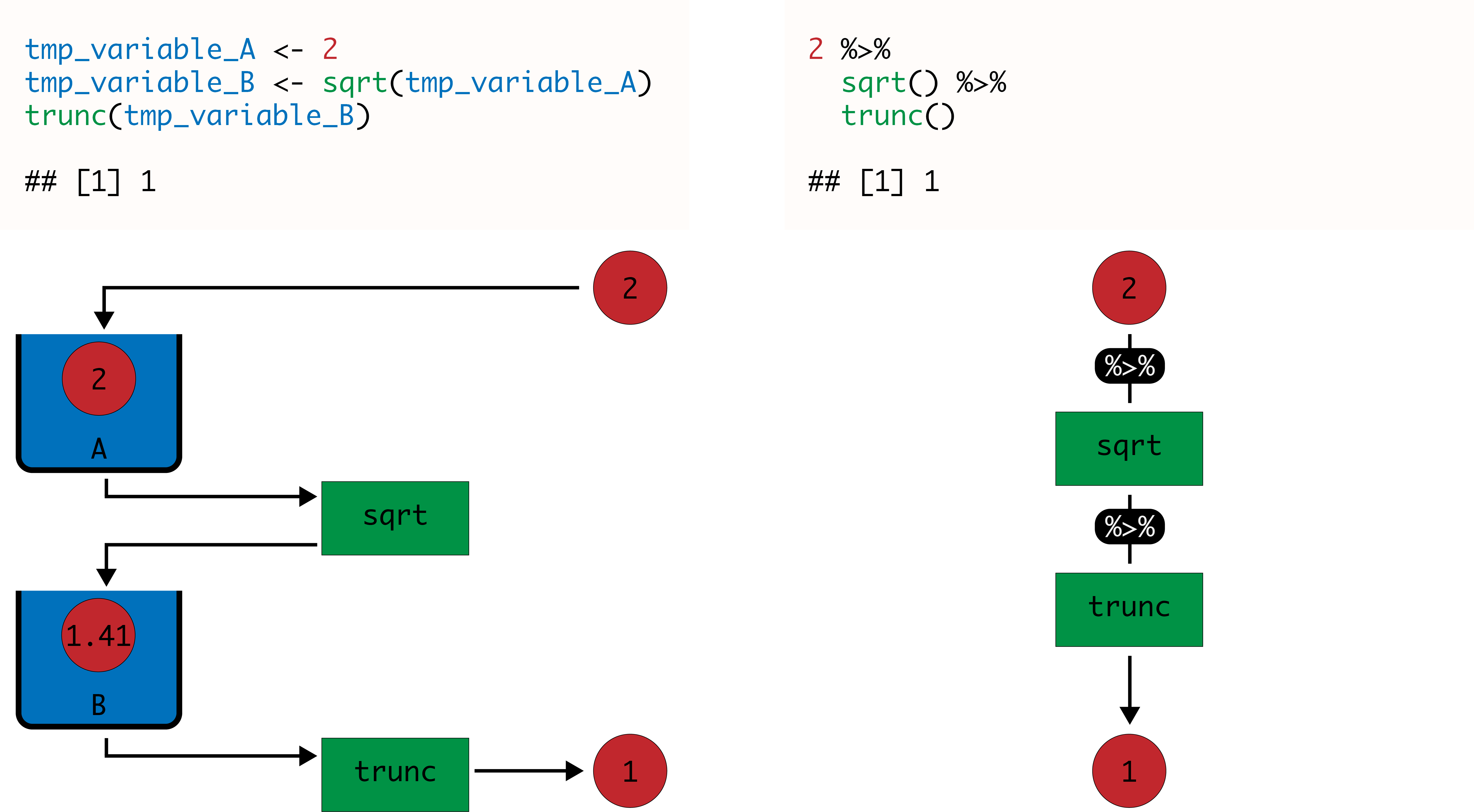
The code below shows a simple example. The number 2 is taken as input for the first pipe that passes it on as the first argument to the function sqrt. The output value 1.41 is then taken as input for the second pipe, which passes it on as the first argument to the function trunc. The final output 1 is finally returned.

2 %>%
  sqrt() %>%
  trunc()

## [1] 1

The image below graphically illustrates how the pipe operator works, compared to the same procedure executed using two temporary variables that are used to store temporary values.

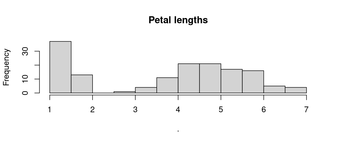
Illustration of how the pipe operator works

Similarly, you can use pipe to recreate the histogram of petal lengths from the iris dataset shown above, using the function pull to extract the column Petal.Length from the table, instead of the operator $. However, the Tidyverse includes the ggplot2 library, which provides support for more sophisticated plotting, as we will see in subsequent chapters.

iris %>% 
  pull(Petal.Length) %>% 
  hist(main = "Petal lengths")

The first step of a sequence of pipes can be a value, a variable, or a function, including arguments. The code below shows a series of examples of different ways of achieving the same result. The examples use the function round, which also allows for a second argument: digits = 2. Note that, when using the pipe operator, only the nominally second argument is provided to the function round – that is round(digits = 2)

# No pipe, using variables
tmp_variable_A <- 2
tmp_variable_B <- sqrt(tmp_variable_A)
round(tmp_variable_B, digits = 2)

# No pipe, using functions only
round(sqrt(2), digits = 2)

# Pipe starting from a value
2 %>%
  sqrt() %>%
  round(digits = 2)

# Pipe starting from a variable
the_value_two <- 2
the_value_two %>%
  sqrt() %>%
  round(digits = 2)

# Pipe starting from a function
sqrt(2) %>%
 round(digits = 2)

A complex operation created through the use of %>% can be used on the right side of <-, to assign the outcome of the operation to a variable.

sqrt_of_two <- 
  2 %>%
  sqrt() %>%
  round(digits = 2)

1.4 Exercise 101.1

Question 101.1.1: Write a piece of code using the pipe operator that takes as input the number 1632, calculates the logarithm to the base 10, takes the highest integer number lower than the calculated value (lower round), and verifies whether it is an integer.

Question 101.1.2: Write a piece of code using the pipe operator that takes as input the number 1632, calculates the square root, takes the lowest integer number higher than the calculated value (higher round), and verifies whether it is an integer.

Question 101.1.3: Write a piece of code using the pipe operator that takes as input the string "1632", transforms it into a number, and checks whether the result is Not a Number.

Question 101.1.4: Write a piece of code using the pipe operator that takes as input the string "-16.32", transforms it into a number, takes the absolute value and truncates it, and finally checks whether the result is Not Available.

Question 101.1.5: Rewrite a piece of code below by substituting the last line with the function mean(). What kind of result do you obtain? What does it represent?

iris %>% 
  pull(Petal.Length) %>% 
  hist(main = "Petal lengths")

Question 101.1.6: Further edit the code created for Question 101.1.6 by substituting Petal.Length with Petal.Width first and Species then? What kind of results do you obtain? What do they mean?

by Stefano De Sabbata – text licensed under the CC BY-SA 4.0, contains public sector information licensed under the Open Government Licence v3.0, code licensed under the GNU GPL v3.0.

Welcome

2 Reproducible data science