10 Supervised machine learning
The field of machine learning sits at the intersection of computer science and statistics, and it is a core component of data science. According to Mitchell (1997), “the field of machine learning is concerned with the question of how to construct computer programs that automatically improve with experience.”
Machine learning approaches are divided into two main types19.
-
Supervised:
- training of a “predictive” model from data;
- one (or more) attribute of the dataset is used to “predict” another attribute.
-
Unsupervised:
- discovery of descriptive patterns in data;
- commonly used in data mining.
Classification is one of the classic supervised machine learning tasks, where algorithms are used to learn (i.e., model) the relationship between a series of input values (a.k.a. predictors, independent variables) and output categorical values or labels (a.k.a. outcome, dependent variable). A model trained on a training dataset can learn the relationship between the input and the labels, and then be used to label new, unlabeled data.
This chapters explores three approaches to supervised machine learning approaches to classification:
- logistic regression;
- support vector machines;
- artificial neural networks.
10.1 Confusion matrices
Once a classification model has been created, the next step is validation. The latter can involve different approaches and procedures, but one of the most common and simple approaches is to split the data between a training and a testing set. The model is trained on the training set and then validated using the testing set. Both sets will contain both the input values (predictors) and the output values (outcome).
The model trained using the training set can be used to predict the values for the testing set. The outcome of the prediction can be compared to the actual categories in the testing dataset. A confusion matrix is a representation of the correspondence between actual values and predicted values in the testing dataset, including:
- true positive: correctly classified as the first (positive) class;
- true negative: correctly classified as the second (negative) class;
- false positive: incorrectly classified as the first (positive) class;
- false negative: incorrectly classified as the second (negative) class.
The number of true and false positive and negatives are used to calculate a number of performance measures. The simplest measures of performance are accuracy and error rate.
\[ accuracy = \frac{true\ positive + true\ negative}{total\ number\ of\ cases} \] \[ error\ rate = 1 - accuracy \]
There are also a number of additional measures that can provide further insight into the quality of the prediction, such as sensitivity (true positive rate) and specificity (true negative rate). If the model has been created to predict a binary categorical variable, based on the definition above (the first category is positive, the second category is negative), sensitivity is a measure of quality in predicting the first category, and specificity is a measure of quality in predicting the second category.
\[ sensitivity = \frac{true\ positive}{true\ positive + false\ negative} = \frac{correct\ 1st}{all\ 1st} \]
\[ specificity = \frac{true\ negative}{true\ negative + false\ positive} = \frac{correct\ 2nd}{all\ 2nd} \]
Two further, similar measures are precision and recall. A model with high precision is a model that can be trusted to make a correct prediction when identifying an observation as being part of the first category. The formula for recall is the same used for sensitivity, but in this case, it has a different interpretation, derived from the computer science literature on search engines, where a model with high recall is able to correctly retrieve most items of the specified category. Note that both precision and recall are dependent on which one of two categories is defined as being the first.
\[ precision = \frac{true\ positive}{true\ positive + false\ positive} = \frac{correct\ 1st}{predicted\ as\ 1st} \]
\[ recall = \frac{true\ positive}{true\ positive + false\ negative} = \frac{correct\ 1st}{all\ 1st} \] Precision and recall can also be combined into a single measure of performance called F-score (a.k.a., F-measure or F1).
\[ F-score = \frac{2 \times precision \times recall}{precision + recall} \] Finally, the kappa statistic (the most common being Cohen’s kappa) is an additional measure of accuracy, which measures the agreement between prediction and actual values, while also accounting for the probability of correct prediction by chance.
10.2 Urban and rural population density
The two examples below explore the relation between some of the variables from the United Kingdom 2011 Census included among the 167 initial variables used to create the 2011 Output Area Classification (Gale et al., 2016) and the Rural Urban Classification (2011) of Output Areas in England and Wales created by the Office for National Statistics. The various examples and models explore whether it is possible to learn the rural-urban distinction by using some of those census variables, in the Local Authority Districts (LADs) in Leicestershire (excluding the city of Leicester itself.
The code below uses the libraries caret, e1071 and neuralnet. Please install them before continuing.
install.packages("caret")
install.packages("e1071")
install.packages("neuralnet")
The examples use the same data seen in previous chapters, but for the 7 LADs in Leicestershire outside the boundaries of the city of Leicester: Blaby, Charnwood, Harborough, Hinckley and Bosworth, Melton, North West Leicestershire, and Oadby and Wigston. Those data are loaded from the 2011_OAC_Raw_uVariables_Leicestershire.csv. The second part of the code extracts the data of the Rural Urban Classification (2011) from the compressed file RUC11_OA11_EW.zip, loads the extracted data and finally deletes them.
# Libraries
library(tidyverse)
library(magrittr)

# 2011 OAC data for Leicestershire (excl. Leicester)
liec_shire_2011OAC <- readr::read_csv("2011_OAC_Raw_uVariables_Leicestershire.csv")

# Rural Urban Classification (2011)
# >>> Note that if you upload the file to RStudio Server
# >>> the file will be automatically unzipped
# >>> thus the unzip and unlink instrcutions are not necessary
unzip("RUC11_OA11_EW.zip")
ru_class_2011 <- readr::read_csv("RUC11_OA11_EW.csv")
unlink("RUC11_OA11_EW.csv")
We can then join the two datasets and create a simplified, binary rural - urban classification, that is used in the examples below.
liec_shire_2011OAC_RU <-
  liec_shire_2011OAC %>%
  dplyr::left_join(ru_class_2011) %>%
  dplyr::mutate(
    rural_urban =
      forcats::fct_recode(
        RUC11CD,
        urban = "C1",
        rural = "D1",
        rural = "E1",
        rural = "F1"
      ) %>%
      forcats::fct_relevel(
        c("rural", "urban")
      )
  )
10.3 Logistic regression
Can we predict whether an Output Area (OA) is urban or rural, solely based on its population density?
liec_shire_2011OAC_RU %>%
  ggplot2::ggplot(
    aes(
      x = u006,
      y = rural_urban
    )
  ) +
  ggplot2::geom_point(
    aes(
      color = rural_urban,
      shape = rural_urban
    )
  ) +
  ggplot2::scale_color_manual(values = c("deepskyblue2", "darkgreen")) +
  ggplot2::scale_x_log10() +
  ggplot2::theme_bw()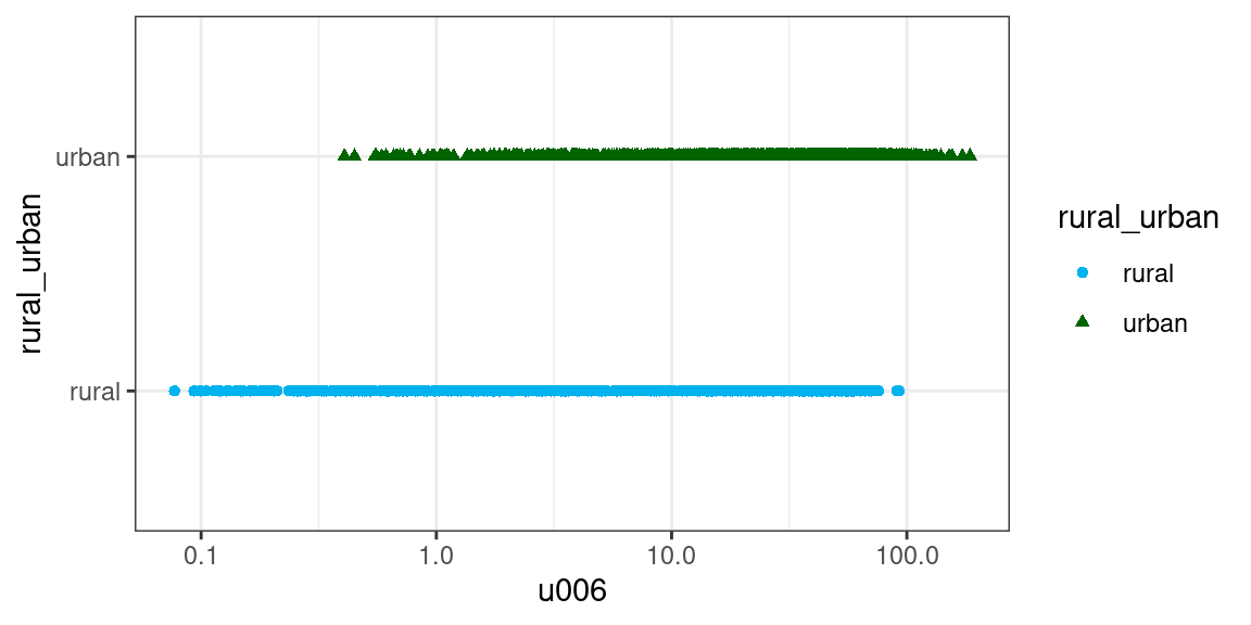
The two patters in the plot above seem quite close even when plotted using a logarithmically transformed x-axis. As a first step, we can extract from the dataset only the data we need, and create a logarithmic transformation of the population density value. To be able to perform a simple validatin our model, we can divide that data in a training (80% of the dataset) and a testing set (20% of the dataset).
# Data for logit model
ru_logit_data <-
  liec_shire_2011OAC_RU %>%
  dplyr::select(OA11CD, u006, rural_urban) %>%
  dplyr::mutate(
    density_log = log10(u006)
  )

# Training set
ru_logit_data_trainig <-
  ru_logit_data %>%
  slice_sample(prop = 0.8)

# Testing set
ru_logit_data_testing <-
  ru_logit_data %>%
  anti_join(ru_logit_data_trainig)
We can then compute the logit model using the stats::glm function and specifying binomial() as family. The summary of the model highlights how the model is significant, but Residual deviance is fairly close to the Null deviance (null model), which is not a good sign.
ru_logit_model <-
  ru_logit_data_trainig %$%
  stats::glm(
    rural_urban ~
      density_log,
    family = binomial()
  )

ru_logit_model %>%
  summary()
##
## Call:
## stats::glm(formula = rural_urban ~ density_log, family = binomial())
##
## Coefficients:
## Estimate Std. Error z value Pr(>|z|)
## (Intercept) -1.23275 0.12739 -9.677 <2e-16 ***
## density_log 1.76297 0.09781 18.025 <2e-16 ***
## ---
## Signif. codes: 0 '***' 0.001 '**' 0.01 '*' 0.05 '.' 0.1 ' ' 1
##
## (Dispersion parameter for binomial family taken to be 1)
##
## Null deviance: 2076.3 on 1667 degrees of freedom
## Residual deviance: 1628.7 on 1666 degrees of freedom
## AIC: 1632.7
##
## Number of Fisher Scoring iterations: 4As per other regression models, it would be necessary to test the assumptions of the logit model and the overall distribution of the residuals. However, as this model only has one predictor, we will confine our performance analysis to simple validation.
We can test the performance of the model through a validation exercise, using the testing dataset. Finally, we can compare the results of the prediction with the original data using a confusion matrix.
ru_logit_prediction <-
  ru_logit_model %>%
  # Use model to predict values
  stats::predict(
    ru_logit_data_testing,
    type = "response"
  ) %>%
  as.numeric()

ru_logit_data_testing <-
  ru_logit_data_testing %>%
  tibble::add_column(
    # Add column with predicted class
    logit_predicted_ru =
      # Values below 0.5 indicate first factor level (rural)
      # Values above 0.5 indicate second factor level (ruban)
      ifelse(
        ru_logit_prediction <= 0.5,
        "rural", # first factor level
        "urban"  # second factor level
      ) %>%
      forcats::as_factor() %>%
      forcats::fct_relevel(
        c("rural", "urban")
      )
  )

# Load library for confusion matrix
library(caret)

# Confusion matrix
caret::confusionMatrix(
  ru_logit_data_testing %>% dplyr::pull(logit_predicted_ru),
  ru_logit_data_testing %>% dplyr::pull(rural_urban),
  mode = "everything"
)
## Confusion Matrix and Statistics
##
## Reference
## Prediction rural urban
## rural 66 21
## urban 56 274
##
## Accuracy : 0.8153
## 95% CI : (0.7747, 0.8514)
## No Information Rate : 0.7074
## P-Value [Acc > NIR] : 2.897e-07
##
## Kappa : 0.5129
##
## Mcnemar's Test P-Value : 0.0001068
##
## Sensitivity : 0.5410
## Specificity : 0.9288
## Pos Pred Value : 0.7586
## Neg Pred Value : 0.8303
## Precision : 0.7586
## Recall : 0.5410
## F1 : 0.6316
## Prevalence : 0.2926
## Detection Rate : 0.1583
## Detection Prevalence : 0.2086
## Balanced Accuracy : 0.7349
##
## 'Positive' Class : rural
## 10.4 Support vector machines
Support vector machines (SVMs) are another very common approach to supervised classification. SVMs perform the classification task by partitioning the data space into regions separated by hyperplanes. For instance, in a bi-dimensional space, a hyperplane is a line, and the algorithm is designed to find the line that best separates two groups of data. Computationally, the process is not dissimilar to linear regression.
To showcase the use of SVMs, the example below expands on the one above by building a model for urban - rural classification that uses total population and area (logarithmically transformed) as two separate input values, rather than combined as population density. The aim of the SVM is then to find a line that maximises the margin between the two groups shown in the plot below.
liec_shire_2011OAC_RU %>%
  ggplot2::ggplot(
    aes(
      x = u006,
      y = Total_Population
    )
  ) +
  ggplot2::geom_point(
    aes(
      color = rural_urban,
      shape = rural_urban
    )
  ) +
  ggplot2::scale_color_manual(values = c("deepskyblue2", "darkgreen")) +
  ggplot2::scale_x_log10() +
  ggplot2::scale_y_log10() +
  ggplot2::theme_bw()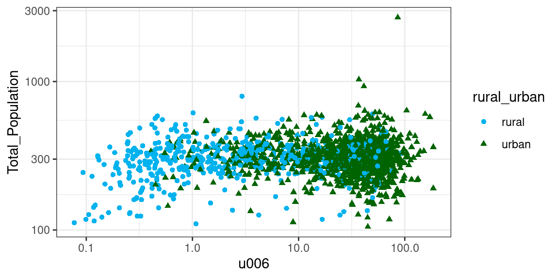
The plot illustrates how the two variables are skewed (note that the axes are logarithmically transformed) and that the two groups are not linearly separable. We can thus follow a procedure similar to the one seen above: extract the necessary data; split the data between training and testing for validation; build the model; predict the values for the testing set and interpret the confusion matrix.
# Data for SVM model
ru_svm_data <-
  liec_shire_2011OAC_RU %>%
  dplyr::select(OA11CD, Total_Population, u006, rural_urban) %>%
  dplyr::mutate(
    area_log = log10(u006),
    population_log = log10(Total_Population)
  )

# Training set
ru_svm_data_trainig <-
  ru_svm_data %>%
  slice_sample(prop = 0.8)

# Testing set
ru_svm_data_testing <-
  ru_svm_data %>%
  anti_join(ru_svm_data_trainig)

# Load library for svm function
library(e1071)

# Build the model
ru_svm_model <-
  ru_svm_data_trainig %$%
  e1071::svm(
    rural_urban ~
      area_log + population_log,
    # Use a simple linear hyperplane
    kernel = "linear",
    # Scale the data
    scale = TRUE,
    # Cost value for observations
    # crossing the hyperplane
    cost = 10
  )

# Predict the values for the testing dataset
ru_svm_prediction <-
  stats::predict(
    ru_svm_model,
    ru_svm_data_testing %>%
      dplyr::select(area_log, population_log)
  )

# Add predicted values to the table
ru_svm_data_testing <-
  ru_svm_data_testing %>%
  tibble::add_column(
    svm_predicted_ru = ru_svm_prediction
  )

# Confusion matrix
caret::confusionMatrix(
  ru_svm_data_testing %>% dplyr::pull(svm_predicted_ru),
  ru_svm_data_testing %>% dplyr::pull(rural_urban),
  mode = "everything"
  )
## Confusion Matrix and Statistics
##
## Reference
## Prediction rural urban
## rural 66 29
## urban 61 261
##
## Accuracy : 0.7842
## 95% CI : (0.7415, 0.8227)
## No Information Rate : 0.6954
## P-Value [Acc > NIR] : 3.136e-05
##
## Kappa : 0.4517
##
## Mcnemar's Test P-Value : 0.001084
##
## Sensitivity : 0.5197
## Specificity : 0.9000
## Pos Pred Value : 0.6947
## Neg Pred Value : 0.8106
## Precision : 0.6947
## Recall : 0.5197
## F1 : 0.5946
## Prevalence : 0.3046
## Detection Rate : 0.1583
## Detection Prevalence : 0.2278
## Balanced Accuracy : 0.7098
##
## 'Positive' Class : rural
## As a third more complex example, we can explore how to build a model for rural - urban classification using the presence of the five different types of dwelling as input variables. The confusion matrix below clearly illustrates that a simple linear SVM is not adequate to construct such a model.
# Data for SVM model
ru_dwellings_data <-
  liec_shire_2011OAC_RU %>%
  dplyr::select(
    OA11CD, rural_urban, Total_Dwellings,
    u086:u090
  ) %>%
  # scale across
  dplyr::mutate(
    dplyr::across(
      u086:u090,
      scale
      #function(x){ (x / Total_Dwellings) * 100 }
    )
  ) %>%
  dplyr::rename(
    scaled_detached = u086,
    scaled_semidetached = u087,
    scaled_terraced = u088,
    scaled_flats = u089,
    scaled_carava_tmp = u090
  ) %>%
  dplyr::select(-Total_Dwellings)

# Training set
ru_dwellings_data_trainig <-
  ru_dwellings_data %>%
  slice_sample(prop = 0.8)

# Testing set
ru_dwellings_data_testing <-
  ru_dwellings_data %>%
  anti_join(ru_dwellings_data_trainig)

# Build the model
ru_dwellings_svm_model <-
  ru_dwellings_data_trainig %$%
  e1071::svm(
    rural_urban ~
      scaled_detached + scaled_semidetached + scaled_terraced +
      scaled_flats + scaled_carava_tmp,
    # Use a simple linear hyperplane
    kernel = "linear",
    # Cost value for observations
    # crossing the hyperplane
    cost = 10
  )

# Predict the values for the testing dataset
ru_dwellings_svm_prediction <-
  stats::predict(
    ru_dwellings_svm_model,
    ru_dwellings_data_testing %>%
      dplyr::select(scaled_detached:scaled_carava_tmp)
  )

# Add predicted values to the table
ru_dwellings_data_testing <-
  ru_dwellings_data_testing %>%
  tibble::add_column(
    dwellings_svm_predicted_ru = ru_dwellings_svm_prediction
  )

# Confusion matrix
caret::confusionMatrix(
  ru_dwellings_data_testing %>% dplyr::pull(dwellings_svm_predicted_ru),
  ru_dwellings_data_testing %>% dplyr::pull(rural_urban),
  mode = "everything"
  )
## Confusion Matrix and Statistics
##
## Reference
## Prediction rural urban
## rural 0 0
## urban 130 287
##
## Accuracy : 0.6882
## 95% CI : (0.6414, 0.7324)
## No Information Rate : 0.6882
## P-Value [Acc > NIR] : 0.5237
##
## Kappa : 0
##
## Mcnemar's Test P-Value : <2e-16
##
## Sensitivity : 0.0000
## Specificity : 1.0000
## Pos Pred Value : NaN
## Neg Pred Value : 0.6882
## Precision : NA
## Recall : 0.0000
## F1 : NA
## Prevalence : 0.3118
## Detection Rate : 0.0000
## Detection Prevalence : 0.0000
## Balanced Accuracy : 0.5000
##
## 'Positive' Class : rural
## 10.4.1 Kernels
Instead of relying on simple linear hyperplanes, we can use the “kernel trick” to project the data into a higher-dimensional space, which might allow groups to be (more easily) linearly separable.
# Build a second model
# using a radial kernel
ru_dwellings_svm_radial_model <-
  ru_dwellings_data_trainig %$%
  e1071::svm(
    rural_urban ~
      scaled_detached + scaled_semidetached + scaled_terraced +
      scaled_flats + scaled_carava_tmp,
    # Use a radial kernel
    kernel = "radial",
    # Cost value for observations
    # crossing the hyperplane
    cost = 10
  )

# Predict the values for the testing dataset
ru_svm_dwellings_radial_prediction <-
  stats::predict(
    ru_dwellings_svm_radial_model,
    ru_dwellings_data_testing %>%
      dplyr::select(scaled_detached:scaled_carava_tmp)
  )

# Add predicted values to the table
ru_dwellings_data_testing <-
  ru_dwellings_data_testing %>%
  tibble::add_column(
    dwellings_radial_predicted_ru = ru_svm_dwellings_radial_prediction
  )

# Confusion matrix
caret::confusionMatrix(
  ru_dwellings_data_testing %>% dplyr::pull(dwellings_radial_predicted_ru),
  ru_dwellings_data_testing %>% dplyr::pull(rural_urban),
  mode = "everything"
  )
## Confusion Matrix and Statistics
##
## Reference
## Prediction rural urban
## rural 29 13
## urban 101 274
##
## Accuracy : 0.7266
## 95% CI : (0.6811, 0.7689)
## No Information Rate : 0.6882
## P-Value [Acc > NIR] : 0.04938
##
## Kappa : 0.2182
##
## Mcnemar's Test P-Value : 3.691e-16
##
## Sensitivity : 0.22308
## Specificity : 0.95470
## Pos Pred Value : 0.69048
## Neg Pred Value : 0.73067
## Precision : 0.69048
## Recall : 0.22308
## F1 : 0.33721
## Prevalence : 0.31175
## Detection Rate : 0.06954
## Detection Prevalence : 0.10072
## Balanced Accuracy : 0.58889
##
## 'Positive' Class : rural
## 10.5 Artificial neural networks
Artificial neural networks (ANNs) are one of the most studied approaches in supervised machine learning, and the term actually defines a large set of different approaches. These model aims to simulate a simplistic version of a brain made of artificial neurons. Each artificial neuron combines a series of input values into one output values, using a series of weights (one per input value) and an activation function. The aim of the model is to learn an optimal set of weights that, once combined with the input values, generates the correct output value. The latter is also influenced by the activation function, which modulates the final result.
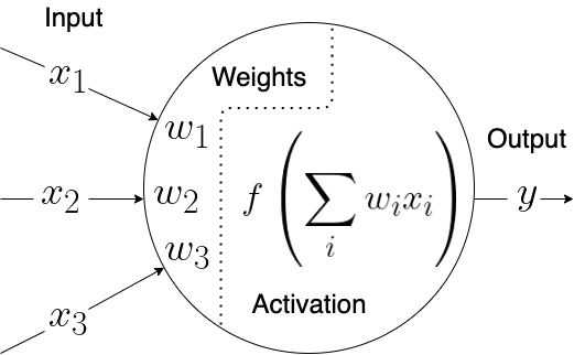
Each neuron is effectively a regression model. The input values are the predictors (or independent variables), the output is the outcome (or dependent variable), and the weights are the coefficients (see also previous chapter on regression models). The selection of the activation function defines the regression model. As ANNs are commonly used for classification, one of the most common activation functions used is the sigmoid, thus rendering every single neuron a logistic regression.
An instance of an ANN is defined by its topology (number of layers and nodes), activation functions and the algorithm used to train the network. The selection of all those parameters renders the construction of ANNs a very complex task, and the quality of the result frequently relies on the experience of the data scientist.
- Number of layers
- Single-layer network: one node of input variable one node per category of the output variable, effectively a logistic regression.
- Multi-layer network: adds one hidden layer, which aims to capture hidden “features” of the data, as combinations of the input values, and use that for the final classification.
- Deep neural networks: several hidden layers, each aiming to capture more and more complex “features” of the data.
- Number of nodes
- The number of nodes needs to be selected for each one of the hidden layers.
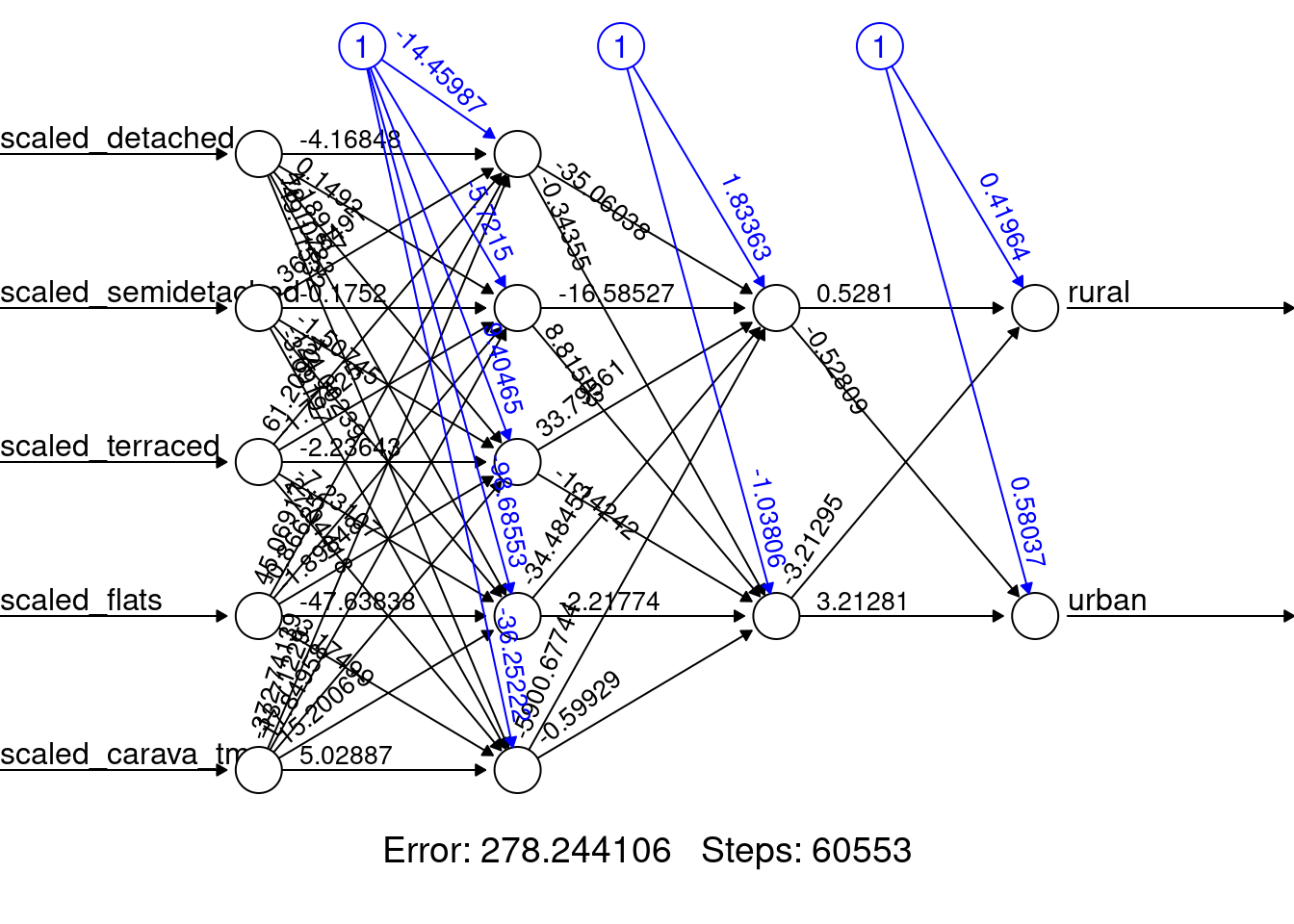
We can explore the construction of an ANN for the same input and output variables seen in the previous example, and compare which one of the two approaches produces better results. The example below creates a multi-layer ANN, using two hidden layers, with five and two nodes, respectively.
# Load library for ANNs
library(neuralnet)

# Build a third model
# using an ANN
ru_dwellings_nnet_model <-
  neuralnet::neuralnet(
    rural_urban ~
      scaled_detached + scaled_semidetached + scaled_terraced +
      scaled_flats + scaled_carava_tmp,
    data = ru_dwellings_data_trainig,
    # Use 2 hidden layers
    hidden = c(5, 2),
    # Max num of steps for training
    stepmax = 1000000
  )
# Predict the values for the testing dataset
ru_dwellings_nnet_prediction <-
  neuralnet::compute(
    ru_dwellings_nnet_model,
    ru_dwellings_data_testing %>%
      dplyr::select(scaled_detached:scaled_carava_tmp)
  )

# Derive predicted categories
ru_dwellings_nnet_predicted_categories <-
  # from the prediction object
  ru_dwellings_nnet_prediction %$%
  # extract the result
  # which is a matrix of probabilities
  # for each object and category
  net.result %>%
  # select the column (thus the category)
  # with higher probability
  max.col %>%
  # recode columns values as
  # rural or urban
  dplyr::recode(
    `1` = "rural",
    `2` = "urban"
  ) %>%
  forcats::as_factor() %>%
  forcats::fct_relevel(
    c("rural", "urban")
  )

# Add predicted values to the table
ru_dwellings_data_testing <-
  ru_dwellings_data_testing %>%
  tibble::add_column(
    dwellings_nnet_predicted_ru =
      ru_dwellings_nnet_predicted_categories
  )

# Confusion matrix
caret::confusionMatrix(
  ru_dwellings_data_testing %>% dplyr::pull(dwellings_nnet_predicted_ru),
  ru_dwellings_data_testing %>% dplyr::pull(rural_urban),
  mode = "everything"
  )
## Confusion Matrix and Statistics
##
## Reference
## Prediction rural urban
## rural 56 24
## urban 74 263
##
## Accuracy : 0.765
## 95% CI : (0.7213, 0.8049)
## No Information Rate : 0.6882
## P-Value [Acc > NIR] : 0.0003257
##
## Kappa : 0.388
##
## Mcnemar's Test P-Value : 7.431e-07
##
## Sensitivity : 0.4308
## Specificity : 0.9164
## Pos Pred Value : 0.7000
## Neg Pred Value : 0.7804
## Precision : 0.7000
## Recall : 0.4308
## F1 : 0.5333
## Prevalence : 0.3118
## Detection Rate : 0.1343
## Detection Prevalence : 0.1918
## Balanced Accuracy : 0.6736
##
## 'Positive' Class : rural
## 10.6 Exercise 404.1
Question 404.1.1: Create an SVM model capable of classifying areas in Leicester and Leicestershire as rural or urban based on the series of variables that relate to “Economic Activity” among the 167 initial variables used to create the 2011 Output Area Classification (Gale et al., 2016).
Question 404.1.2: Create an ANN using the same input and output values used in Question 404.1.1.
Question 404.1.3: Assess which one of the two models preforms a better classification.
by Stef De Sabbata – text licensed under the CC BY-SA 4.0, contains public sector information licensed under the Open Government Licence v3.0, code licensed under the GNU GPL v3.0.