Solutions

Solutions 101

Note that you can add sections to your code, such as the “Intro” section below by selecting Code > Insert Section… from the top menu in RStudio. Those will then be visible on a right panel in the RStudio integrated editor if you select Code > Show Document Outline from the top menu. Code sections can help to visually organise your code and the Document Outline allows you to select a section and jump to it in the code.

The code below deletes all variable and function currently defined in the environment, which is generally good practice, to avoid your script interacting with objects left over from previous sessions.

rm(list = ls())

Load the necessary libraries.

# Load the tidyverse
library(tidyverse)

# Load magrittr
# necessary for options 3 and 4 
# of my answer to Question 101.2.4
library(magrittr)

Solutions 101.1

Question 101.1.1: Write a piece of code using the pipe operator that takes as input the number 1632, calculates the logarithm to the base 10, takes the highest integer number lower than the calculated value (lower round), and verifies whether it is an integer.

1632 %>%
  # calculate the logarithm to the base 10
  log10() %>%
  # highest integer number lower than the value
  floor() %>%
  # check whether it is an integer
  is.integer()
  # The answer is FALSE
  # as the value is still of type numeric
  # rather than type integer

# The code below replicates the procedure above
# but checking the value data type
1632 %>%
  log10() %>%
  floor() %>%
  class()

# The code below replicates the procedure above
# but using as.integer to transfor the value
# to an integer type
1632 %>%
  log10() %>%
  floor() %>%
  as.integer() %>%
  class()

# As above but checking whether the value is an integer
1632 %>%
  log10() %>%
  floor() %>%
  as.integer() %>%
  is.integer()

Question 101.1.2: Write a piece of code using the pipe operator that takes as input the number 1632, calculates the square root, takes the lowest integer number higher than the calculated value (higher round), and verifies whether it is an integer.

1632 %>%
  # calculate the square root
  sqrt() %>%
  # lowest integer number higher than the value
  ceiling() %>%
  # check whether it is an integer
  is.integer()

Question 101.1.3: Write a piece of code using the pipe operator that takes as input the string "1632", transforms it into a number, and checks whether the result is Not a Number.

"1632" %>%
  # transform it into a number
  as.numeric() %>%
  # check whether the result is Not a Number
  is.nan()

Question 101.1.4: Write a piece of code using the pipe operator that takes as input the string "-16.32", transforms it into a number, takes the absolute value and truncates it, and finally checks whether the result is Not Available.

"-16.32" %>%
  # transform it into a number
  as.numeric() %>%
  # take the absolute value
  abs() %>%
  # truncate
  trunc() %>%
  # check whether the result is Not Available
  is.na()

Question 101.1.5: Rewrite a piece of code below by substituting the last line with the function mean(). What kind of result do you obtain? What does it represent?

iris %>% 
  pull(Petal.Length) %>% 
  mean()

The output is a numeric value representing the aritmetic mean (average) of all the petal lengths of flowers in the iris dataset.

Question 101.1.6: Further edit the code created for Question 101.1.6 by substituting Petal.Length with Petal.Width first and Species then? What kind of results do you obtain? What do they mean?

iris %>% 
  pull(Petal.Width) %>% 
  mean()

iris %>% 
  pull(Species) %>% 
  mean()

Solutions 102

Solutions 102.1

Extend the code in the script practical-102_my-script-002.R to include the code necessary to solve the questions below.

library(tidyverse)
library(nycflights13)
library(knitr)

Question 101.1.1: Write a piece of code using the pipe operator and the dplyr library to generate a table showing the air time and the carrier, but only for flights starting from the JFK airport. As in the examples above, use slice_head and kable to output a nicely-formatted table containing only the first 10 rows.

# Start from the entire dataset
flights %>%
  # Retain only the necessary columns
  select(origin, carrier, air_time) %>%
  # Retain only rows representing flights from JFK
  filter(origin == "JFK") %>%
  slice_head(n = 5) %>%
  kable()

origin	carrier	air_time
JFK	AA	160
JFK	B6	183
JFK	B6	140
JFK	B6	149
JFK	B6	158

Question 102.1.2: Write a piece of code using the pipe operator and the dplyr library to generate a table showing the arrival delay and the overall air time, but only for flights of October 12th. As in the examples above, use slice_head and kable to output a nicely-formatted table containing only the first 10 rows.

# Start from the entire dataset
flights %>%
  # Retain only the necessary columns
  select(year:day, arr_delay, air_time) %>%
  # Retain only rows where month equals 10 and day equals 12
  filter(month == 10 & day == 12) %>%
  slice_head(n = 5) %>%
  kable()

year	month	day	arr_delay	air_time
2013	10	12	-20	74
2013	10	12	-27	181
2013	10	12	-30	142
2013	10	12	-10	193
2013	10	12	17	210

Question 102.1.3: Write a piece of code using the pipe operator and the dplyr library to generate a table showing the arrival delay, origin and destination, but only for flight leaving between 11am and 2pm. As in the examples above, use slice_head and kable to output a nicely-formatted table containing only the first 10 rows.

# Start from the entire dataset
flights %>%
  # Retain only the necessary columns
  select(origin, dest, dep_time, arr_delay) %>%
  # Retain only rows where departure time is greater than or equal to 1100
  # and departure time is also less than or equal to 1100
  filter(dep_time >= 1100 & dep_time <= 1400) %>%
  slice_head(n = 5) %>%
  kable()

origin	dest	dep_time	arr_delay
EWR	PBI	1101	13
LGA	MIA	1103	-11
EWR	SFO	1105	23
LGA	CMH	1107	-5
LGA	MIA	1109	-23

Solutions 103

Solutions 103.1

Create an RMarkdown document in RStudio, using Exercise 103 as title and PDF as output. Delete all the contents except the first five lines which compose the heading. Save the document as practical-103_exercises.Rmd. Add the libraries and code necessary to read the data from the 2011_OAC_Raw_uVariables_Leicester.csv file. Create a first section of the document (e.g., adding a second heading Exercise 103.1) and add your answers to the questions below.

In order to answer the questions below, inspect the look-up table 2011_OAC_Raw_uVariables_Lookup.csv (e.g., using Microsoft Excel) to identify the columns necessary to complete the task.

Question 103.1.1: Identify the five variables which are part of the variable subdomain Housing Type and write the code necessary to compute the total number of household spaces in Leicester for each housing type.

leicester_2011OAC %>% 
  summarise(
    u086_tot = sum(u086),
    u087_tot = sum(u087),
    u088_tot = sum(u088),
    u089_tot = sum(u089),
    u090_tot = sum(u090)
  ) %>% 
  kable()

u086_tot	u087_tot	u088_tot	u089_tot	u090_tot
13390	44880	40290	28757	66

Question 103.1.2: Write the code necessary to compute the total number of household spaces in Leicester for each housing type grouped by 2011 OAC supergroup.

leicester_2011OAC %>% 
  group_by(supgrpname) %>% 
  summarise(
    u086_tot = sum(u086),
    u087_tot = sum(u087),
    u088_tot = sum(u088),
    u089_tot = sum(u089),
    u090_tot = sum(u090)
  ) %>% 
  kable()

supgrpname	u086_tot	u087_tot	u088_tot	u089_tot	u090_tot
Constrained City Dwellers	176	1495	941	1876	3
Cosmopolitans	296	580	3185	7261	3
Ethnicity Central	187	465	1292	7093	6
Hard-Pressed Living	618	7825	3891	370	13
Multicultural Metropolitans	7700	26940	28804	10990	40
Suburbanites	2458	3852	210	111	0
Urbanites	1955	3723	1967	1056	1

Question 103.1.3: Write the code necessary to compute the percentage of household spaces (i.e., over to the total number of household spaces) in Leicester for each housing type grouped by 2011 OAC supergroup.

leicester_2011OAC %>% 
  group_by(supgrpname) %>% 
  summarise(
    u086_tot = sum(u086),
    u087_tot = sum(u087),
    u088_tot = sum(u088),
    u089_tot = sum(u089),
    u090_tot = sum(u090)
  ) %>% 
  mutate(
    tot_hspaces = 
      u086_tot + u087_tot +
      u088_tot + u089_tot +
      u090_tot
  ) %>% 
  mutate(
    u086_perc = (u086_tot / tot_hspaces) * 100,
    u087_perc = (u087_tot / tot_hspaces) * 100,
    u088_perc = (u088_tot / tot_hspaces) * 100,
    u089_perc = (u089_tot / tot_hspaces) * 100,
    u090_perc = (u090_tot / tot_hspaces) * 100
  ) %>% 
  select(
    supgrpname,
    u086_perc, u087_perc, u088_perc,
    u089_perc, u090_perc
  ) %>% 
  kable(digits = c(0, 2, 2, 2, 2, 2))

supgrpname	u086_perc	u087_perc	u088_perc	u089_perc	u090_perc
Constrained City Dwellers	3.92	33.29	20.95	41.77	0.07
Cosmopolitans	2.61	5.12	28.12	64.11	0.03
Ethnicity Central	2.07	5.14	14.29	78.44	0.07
Hard-Pressed Living	4.86	61.53	30.60	2.91	0.10
Multicultural Metropolitans	10.34	36.17	38.68	14.76	0.05
Suburbanites	37.07	58.09	3.17	1.67	0.00
Urbanites	22.47	42.78	22.60	12.14	0.01

Question 103.1.4: Modify the code written for Question 103.1.3, using the verb rename to change the column names of the columns containing the percentages to names that resemble the related housing type (e.g., perc_of_detached).

Solutions 104

Solutions 104.1

Extend the code in the script Data_Wrangling_Example.R (see code below) to include the code necessary to solve the questions below. Use the full list of variable names from the 2011 UK Census used to generate the 2011 OAC thatcan be found in the file 2011_OAC_Raw_uVariables_Lookup.csv to indetify which columns to use to complete the tasks.

# Data_Wrangling_Example.R 

# Load the tidyverse
library(tidyverse)

# Load 2011 OAC data
leicester_2011OAC <- 
  read_csv("data/2011_OAC_Raw_uVariables_Leicester.csv")

# Load Indexes of Multiple deprivation data
leicester_IMD2015 <- 
  read_csv("data/IndexesMultipleDeprivation2015_Leicester.csv")

leicester_IMD2015_decile_wide <- leicester_IMD2015 %>%
  # Select only Socres
  filter(Measurement == "Decile") %>%
  # Trim names of IndicesOfDeprivation
  mutate(
    IndicesOfDeprivation = str_replace_all(IndicesOfDeprivation, "\\s", "")
  ) %>%
  mutate(
    IndicesOfDeprivation = str_replace_all(IndicesOfDeprivation, "[:punct:]", "")
  ) %>%
  mutate(
    IndicesOfDeprivation = str_replace_all(IndicesOfDeprivation, "\\(", "")
  ) %>%
  mutate(
    IndicesOfDeprivation = str_replace_all(IndicesOfDeprivation, "\\)", "")
  ) %>%
  # Spread
  pivot_wider(
    names_from = IndicesOfDeprivation,
    values_from = Value
  ) %>%
  # Drop columns
  select(-DateCode, -Measurement, -Units)

# Join
leicester_2011OAC_IMD2015 <- 
  leicester_2011OAC %>%
  inner_join(
    leicester_IMD2015_decile_wide, 
    by = c("LSOA11CD" = "FeatureCode")
  )

Question 104.1.1: Write a piece of code using the pipe operator and the dplyr library to generate a table showing the percentage of EU citizens over total population, calculated grouping OAs by the related decile of the Index of Multiple Deprivations, but only accounting for areas classified as Cosmopolitans or Ethnicity Central or Multicultural Metropolitans.

leicester_2011OAC_IMD2015 %>%
  filter(supgrpname %in% c("Cosmopolitans", "Ethnicity Central", "Multicultural Metropolitans")) %>%
  group_by(IndexofMultipleDeprivationIMD) %>%
  summarise(
    adults_not_empl_perc = (sum(u044 + u045) / sum(Total_Population)) * 100
  ) %>%
  kable()

Question 104.1.2: Write a piece of code using the pipe operator and the dplyr library to generate a table showing the percentage of EU citizens over total population, calculated grouping OAs by the related supergroup in the 2011 OAC, but only accounting for areas in the top 5 deciles of the Index of Multiple Deprivations.

leicester_2011OAC_IMD2015 %>%
  filter(IndexofMultipleDeprivationIMD <= 5) %>%
  group_by(supgrpname) %>%
  summarise(
    eu_perc = (sum(u043 + u044 + u045) / sum(Total_Population)) * 100
  ) %>%
  kable()

Question 104.1.3: Write a piece of code using the pipe operator and the dplyr library to generate a table showing the percentage of people aged 65 and above, calculated grouping OAs by the related supergroup in the 2011 OAC and decile of the Index of Multiple Deprivations, and ordering the table by the calculated value in a descending order.

leicester_2011OAC_IMD2015 %>%
  filter(IndexofMultipleDeprivationIMD <= 5) %>%
  group_by(supgrpname, IndexofMultipleDeprivationIMD) %>%
  summarise(
    aged_65_above = (sum(u016 + u017 + u018 + u019) / sum(Total_Population)) * 100
  ) %>%
  arrange(-aged_65_above) %>%
  kable()

Extend the code in the script Data_Wrangling_Example.R to include the code necessary to solve the questions below.

Question 104.1.4: Write a piece of code using the pipe operator and the dplyr and tidyr libraries to generate a long format of the leicester_2011OAC_IMD2015 table only including the values (census variables) used in Question 104.1.3.

long_table <- leicester_2011OAC_IMD2015 %>%
  select(OA11CD, supgrpname, IndexofMultipleDeprivationIMD, u016, u017, u018, u019, Total_Population) %>%
  pivot_longer(
    # Can't combine character values (e.g. supgrpname)
    # with numeric value (e.g, Total_Population) thus
    # pivot only numeric columns
    cols = u016:Total_Population,
    names_to = "attribute",
    values_to = "value"
  ) 

long_table %>%
  slice_head(n = 5) %>%
  kable()

long_table_alt <- leicester_2011OAC_IMD2015 %>%
  select(OA11CD, supgrpcode, IndexofMultipleDeprivationIMD, u016, u017, u018, u019, Total_Population) %>%
  pivot_longer(
    # Otherwise, use supgrpcode instead of supgrpname
    cols = -OA11CD,
    names_to = "attribute",
    values_to = "value"
  ) 

long_table_alt %>%
  slice_head(n = 7) %>%
  kable()

Question 104.1.5: Write a piece of code using the pipe operator and the dplyr and tidyr libraries to generate a table similar to the one generated for Question 104.1.4, but showing the values as percentages over total population.

perc_long_table <- leicester_2011OAC_IMD2015 %>%
  select(OA11CD, supgrpname, IndexofMultipleDeprivationIMD, u016, u017, u018, u019, Total_Population) %>%
  mutate(
    perc_u016 = (u016 / Total_Population) * 100, 
    perc_u017 = (u017 / Total_Population) * 100, 
    perc_u018 = (u018 / Total_Population) * 100, 
    perc_u019 = (u019 / Total_Population) * 100
  ) %>%
  select(OA11CD, supgrpname, IndexofMultipleDeprivationIMD, perc_u016, perc_u017, perc_u018, perc_u019) %>%
  pivot_longer(
    # Can't combine character values (e.g. supgrpname)
    # with numeric value (e.g, Total_Population) thus
    # pivot only numeric columns
    cols = perc_u016:perc_u019,
    names_to = "attribute",
    values_to = "value"
  ) 

perc_long_table %>%
  slice_head(n = 5) %>%
  kable()

Solutions 201

Solutions 201.1

Open the Leicester_population project used in previous chapters and extend the “Exploring deprivation indices in Leicester” document to include the code necessary to solve the questions below. Use the full list of variable names from the 2011 UK Census used to generate the 2011 OAC that can be found in the file 2011_OAC_Raw_uVariables_Lookup.csv to indetify which columns to use to complete the tasks.

Question 201.1.1: Write a piece of code to create a chart showing the percentage of EU citizens over total population for each decile of the Index of Multiple Deprivations

leicester_2011OAC_IMD2015 %>% 
  group_by(IndexofMultipleDeprivationIMD) %>%
  summarise(
    eu_perc = (sum(u043 + u044 + u045) / sum(Total_Population)) * 100
  ) %>%
  ggplot(
    aes(
      x = eu_perc,
      # Note that it is necessary to convert the index
      # to a factor, otherwise it is interpreted as a number
      y = as_factor(IndexofMultipleDeprivationIMD)
    )
  ) +
  geom_col() +
  theme_bw()

Alternatively.

leicester_2011OAC_IMD2015 %>% 
  group_by(IndexofMultipleDeprivationIMD) %>%
  summarise(
    eu_perc = (sum(u043 + u044 + u045) / sum(Total_Population)) * 100
  ) %>%
  mutate(
    reminder = 100 - eu_perc
  ) %>%
  pivot_longer(
    cols = -IndexofMultipleDeprivationIMD,
    names_to = "country_of_origin",
    values_to = "percentage"
  ) %>% 
  ggplot(
    aes(
      x = percentage,
      # Note that it is necessary to convert the index
      # to a factor, otherwise it is interpreted as a number
      y = as_factor(IndexofMultipleDeprivationIMD),
      fill = country_of_origin
    )
  ) +
  geom_col() +
  theme_bw()

Question 201.1.2: Write a piece of code to create a chart showing the relationship between the percentage of EU citizens over total population with the related score of the Index of Multiple Deprivations, and illustrating also the 2011 OAC class of each OA.

# Use a similar code as used in Exercise 104
# but filtering in the Scores rather than the deciles
leicester_IMD2015_score_wide <- leicester_IMD2015 %>%
  # Select only Socres
  filter(Measurement == "Score") %>%
  # Trim names of IndicesOfDeprivation
  mutate(
    IndicesOfDeprivation = str_replace_all(IndicesOfDeprivation, "\\s", "")
  ) %>%
  mutate(
    IndicesOfDeprivation = str_replace_all(IndicesOfDeprivation, "[:punct:]", "")
  ) %>%
  mutate(
    IndicesOfDeprivation = str_replace_all(IndicesOfDeprivation, "\\(", "")
  ) %>%
  mutate(
    IndicesOfDeprivation = str_replace_all(IndicesOfDeprivation, "\\)", "")
  ) %>%
  # Spread
  pivot_wider(
    names_from = IndicesOfDeprivation,
    values_from = Value
  ) %>%
  # Drop columns
  select(-DateCode, -Measurement, -Units)

# Join
leicester_2011OAC_IMD2015_score <- 
  leicester_2011OAC %>%
  inner_join(
    leicester_IMD2015_score_wide, 
    by = c("LSOA11CD" = "FeatureCode")
  )

leicester_2011OAC_IMD2015_score %>% 
  mutate(
    eu_perc = ((u043 + u044 + u045) / Total_Population) * 100
  ) %>%
  ggplot(
    aes(
      x = eu_perc,
      y = IndexofMultipleDeprivationIMD,
      colour = fct_reorder(supgrpname, supgrpcode)
    )
  ) +
  geom_point() +
  scale_fill_manual(
    values = c("#e41a1c", "#f781bf", "#ff7f00", "#a65628", "#984ea3", "#377eb8", "#ffff33")
  ) +
  theme_bw()

Question 201.1.3: Write a piece of code to create a chart showing the relationship between the percentage of people aged 65 and above with the related score of the Income Deprivation, and illustrating also the 2011 OAC class of each OA.

leicester_2011OAC_IMD2015_score %>% 
  mutate(
    aged_65_above = ((u016 + u017 + u018 + u019) / Total_Population) * 100
  ) %>%
  ggplot(
    aes(
      x = aged_65_above,
      y = LivingEnvironmentDeprivationDomain,
      colour = fct_reorder(supgrpname, supgrpcode)
    )
  ) +
  geom_point() +
  scale_fill_manual(
    values = c("#e41a1c", "#f781bf", "#ff7f00", "#a65628", "#984ea3", "#377eb8", "#ffff33")
  ) +
  theme_bw()

Question 201.1.4: What does the graph produced for Question 201.1.3 mean? Write up to 100 words explaining what conclusions can be drawn from the graph – remember that “the larger the score, the more deprived the area”.

Question 201.1.5: Identify the index of multiple deprivation that most closely relate to the percentage of people per OA whose “day-to-day activities limited a lot or a little” based on the “Standardised Illness Ratio”.

Solutions 202

Solutions 202.1

Create a new RMarkdown document, and add the code necessary to recreate the table leic_2011OAC_20to24 used in the example above. Use the code below to re-shape the table leic_2011OAC_20to24 by pivoting the perc_age_20_to_24 column wider into multiple columns using supgrpname as new column names.

leic_2011OAC_20to24_supgrp <- leic_2011OAC_20to24 %>%
  pivot_wider(
    names_from = supgrpname,
    values_from = perc_age_20_to_24
  )

That manipulation creates one column per supergroup, containing the perc_age_20_to_24 if the OA is part of that supergroup, or an NA value if the OA is not part of the supergroup. The transformation is illustrated in the two tables below. The first shows an extract from the original leic_2011OAC_20to24 dataset, followed by the wide version leic_2011OAC_20to24_supgrp.

leic_2011OAC_20to24 %>%
  slice_min(OA11CD, n = 10) %>%
  kable(digits = 3)

OA11CD	supgrpname	perc_age_20_to_24
E00068657	HP	6.053
E00068658	MM	6.964
E00068659	MM	8.383
E00068660	MM	4.643
E00068661	MM	10.625
E00068662	MM	8.284
E00068663	MM	8.357
E00068664	MM	3.597
E00068665	MM	7.068
E00068666	MM	5.864

leic_2011OAC_20to24_supgrp %>%
  slice_min(OA11CD, n = 10) %>%
  kable(digits = 3)

OA11CD	SU	CP	MM	EC	CD	HP	UR
E00068657	NA	NA	NA	NA	NA	6.053	NA
E00068658	NA	NA	6.964	NA	NA	NA	NA
E00068659	NA	NA	8.383	NA	NA	NA	NA
E00068660	NA	NA	4.643	NA	NA	NA	NA
E00068661	NA	NA	10.625	NA	NA	NA	NA
E00068662	NA	NA	8.284	NA	NA	NA	NA
E00068663	NA	NA	8.357	NA	NA	NA	NA
E00068664	NA	NA	3.597	NA	NA	NA	NA
E00068665	NA	NA	7.068	NA	NA	NA	NA
E00068666	NA	NA	5.864	NA	NA	NA	NA

Question 202.1.1: The code below uses the newly created leic_2011OAC_20to24_supgrp table to calculate the descriptive statistics calculated for the variable leic_2011OAC_20to24 for each supergroup. Is leic_2011OAC_20to24 normally distributed in any of the subgroups? If yes, which supergroups and based on which values do you justify that claim? (Write up to 200 words)

leic_2011OAC_20to24_supgrp %>%
  select(-OA11CD) %>%
  stat.desc(norm = TRUE) %>%
  kable(digits = 3)

	SU	CP	MM	EC	CD	HP	UR
nbr.val	54.000	83.000	573.000	57.000	36.000	101.000	65.000
nbr.null	0.000	0.000	0.000	0.000	0.000	0.000	0.000
nbr.na	915.000	886.000	396.000	912.000	933.000	868.000	904.000
min	1.462	3.141	2.490	2.066	1.064	1.515	2.256
max	9.562	60.751	52.507	36.299	12.963	11.261	13.505
range	8.100	57.609	50.018	34.233	11.899	9.746	11.249
sum	295.867	2646.551	5214.286	838.415	252.108	619.266	372.010
median	5.476	30.457	7.880	10.881	6.854	6.053	5.380
mean	5.479	31.886	9.100	14.709	7.003	6.131	5.723
SE.mean	0.233	1.574	0.230	1.373	0.471	0.172	0.264
CI.mean.0.95	0.467	3.131	0.452	2.751	0.956	0.341	0.528
var	2.929	205.556	30.285	107.523	7.983	2.980	4.545
std.dev	1.712	14.337	5.503	10.369	2.825	1.726	2.132
coef.var	0.312	0.450	0.605	0.705	0.403	0.282	0.372
skewness	0.005	0.067	3.320	0.633	0.322	0.124	1.042
skew.2SE	0.008	0.127	16.266	1.001	0.410	0.258	1.753
kurtosis	-0.391	-0.825	15.143	-1.009	-0.142	0.220	1.441
kurt.2SE	-0.306	-0.789	37.156	-0.810	-0.093	0.231	1.229
normtest.W	0.991	0.980	0.684	0.889	0.965	0.993	0.937
normtest.p	0.954	0.239	0.000	0.000	0.310	0.886	0.002

We can set a p < .01 threshold, which is reasonable for the number of cases in the dataset (hundreds, at least for some of the 2011OAC supergroups). We can claim that leic_2011OAC_20to24 is normally distributed in the supergroups Suburbanites (SU), Cosmopolitans (CP), Constrained City Dwellers (CD) and Hard-Pressed Living (HP), as the normtest.p value is above 0.01, which allows us to reject the null hypothesis. The variable leic_2011OAC_20to24 seems instead not to be normally distributed for Multicultural Metropolitans (MM), Ethnicity Central (EC) and Urbanites (UR). That is also further illustrated by the graphs below.

leic_2011OAC_20to24 %>% 
  filter(supgrpname %in% c("SU", "CP", "CD", "HP")) %>% 
  ggplot(
    aes(
      x = perc_age_20_to_24
    )
  ) + 
  geom_histogram(
    aes(
      y = ..density..
    )
  ) +
  facet_wrap(
    vars(supgrpname),
    ncol = 2,
    scales = "free"
  ) +
  ggtitle("Normally distributed") +
  theme_bw()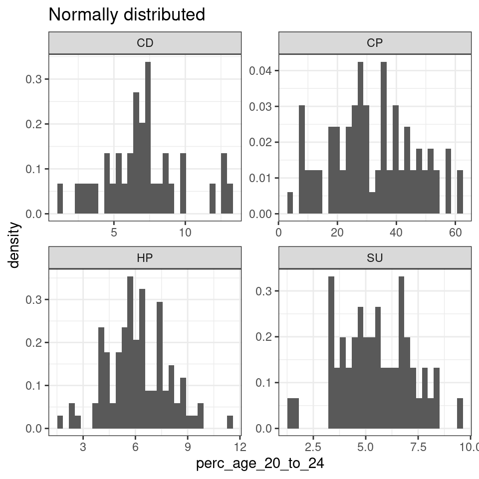

leic_2011OAC_20to24 %>% 
  filter(supgrpname %in% c("MM", "EC", "UR")) %>% 
  ggplot(
    aes(
      x = perc_age_20_to_24
    )
  ) + 
  geom_histogram(
    aes(
      y = ..density..
    )
  ) +
  facet_wrap(
    vars(supgrpname),
    ncol = 2,
    scales = "free"
  ) +
  ggtitle("Not normally distributed") +
  theme_bw()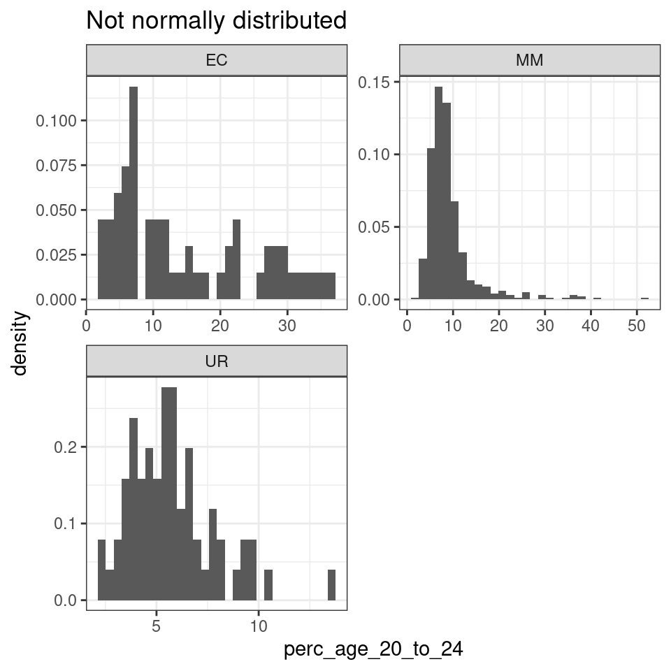

Question 202.1.2: Write the code necessary to test again the normality of leic_2011OAC_20to24 for the supergroups where the analysis conducted for Question 202.1.1 indicated they are normal, using the function shapiro.test, and draw the respective Q-Q plot.

Example for Hard-Pressed Living (HP).

leic_2011OAC_20to24 %>%
  filter(supgrpname == "HP") %>% 
  pull(perc_age_20_to_24) %>%
  shapiro.test()

## 
##  Shapiro-Wilk normality test
## 
## data:  .
## W = 0.99303, p-value = 0.8863

leic_2011OAC_20to24 %>%
  filter(supgrpname == "HP") %>% 
  ggplot(
    aes(
      sample = perc_age_20_to_24
    )
  ) +
  stat_qq() +
  stat_qq_line()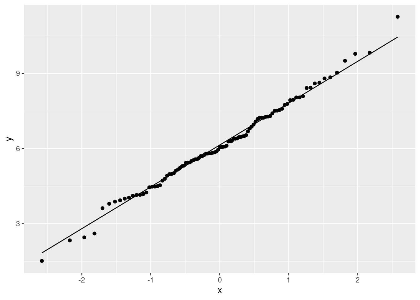

Question 202.1.3: Observe the output of the Levene’s test executed below. What does the result tell you about the variance of perc_age_20_to_24 in supergroups?

Note that the leveneTest was not designed to work with a Tidyverse approach. As such, the code below uses the . argument placeholder to specify that the input table leic_2011OAC_20to24 which is coming down from the pipe should be used as argument for the data parameter.

leic_2011OAC_20to24 %>% 
  leveneTest(
    perc_age_20_to_24 ~ supgrpname, 
    data = .
  )

## Levene's Test for Homogeneity of Variance (center = median)
##        Df F value    Pr(>F)    
## group   6  62.011 < 2.2e-16 ***
##       962                      
## ---
## Signif. codes:  0 '***' 0.001 '**' 0.01 '*' 0.05 '.' 0.1 ' ' 1

If significant, the Levene’s test indicates that the variance is different in different levels. As before, we can set a p < .01 threshold. In the output above, the p value (Pr(>F)) is much lower than our threshold, indicating that the test is significance. Thus, the perc_age_20_to_24 has different variance for different 2011OAc supergroups.

Solutions 203

Solutions 203.1

Create a new RMarkdown document, and add the code necessary to oad the 2011_OAC_Raw_uVariables_Leicester.csv dataset.

library(tidyverse)
library(magrittr)
library(knitr)
library(pastecs)

leicester_2011OAC <- read_csv("2011_OAC_Raw_uVariables_Leicester.csv")

Question 203.1.1: Check whether the values of mean age (u020) are normally distributed, and whether they can be transformed into a normally distributed set using logarithmic or inverse hyperbolic sine functions.

Start from exploring the variable distribution.

leicester_2011OAC %>% 
  ggplot(aes(
    x = u020
  )) +
  geom_histogram() +
  theme_bw()

## `stat_bin()` using `bins = 30`. Pick better value with `binwidth`.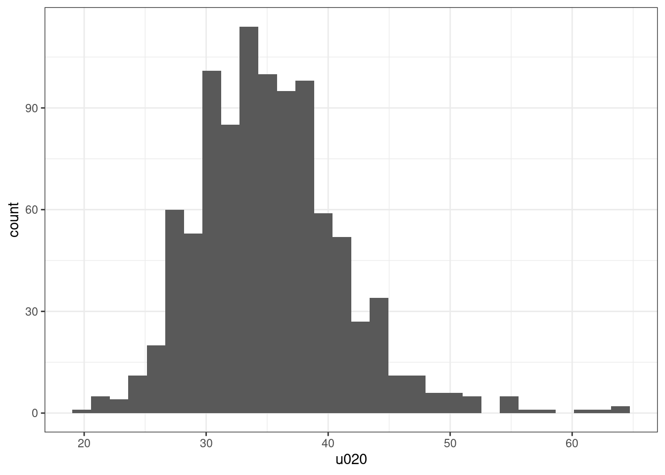

leicester_2011OAC %>% 
  ggplot(aes(
    sample = u020
  )) +
  stat_qq() +
  stat_qq_line() +
  theme_bw()

leicester_2011OAC %>% 
  pull(u020) %>% 
  shapiro.test()

## 
##  Shapiro-Wilk normality test
## 
## data:  .
## W = 0.9663, p-value = 3.476e-14

The variable u020 is clearly not normally distributed, probably mostly due to a long tail on the right side.

Thus, we can try transform the variable using a logarithmic transformation or a inverse hyperbolic sine transformation. Let’s try both.

leicester_2011OAC_trans <-
  leicester_2011OAC %>% 
  mutate(
    log10_u020 = log10(u020),
    ihs_u020 = asinh(u020)
  )

leicester_2011OAC_trans %>% 
  ggplot(aes(
    sample = log10_u020
  )) +
  stat_qq() +
  stat_qq_line() +
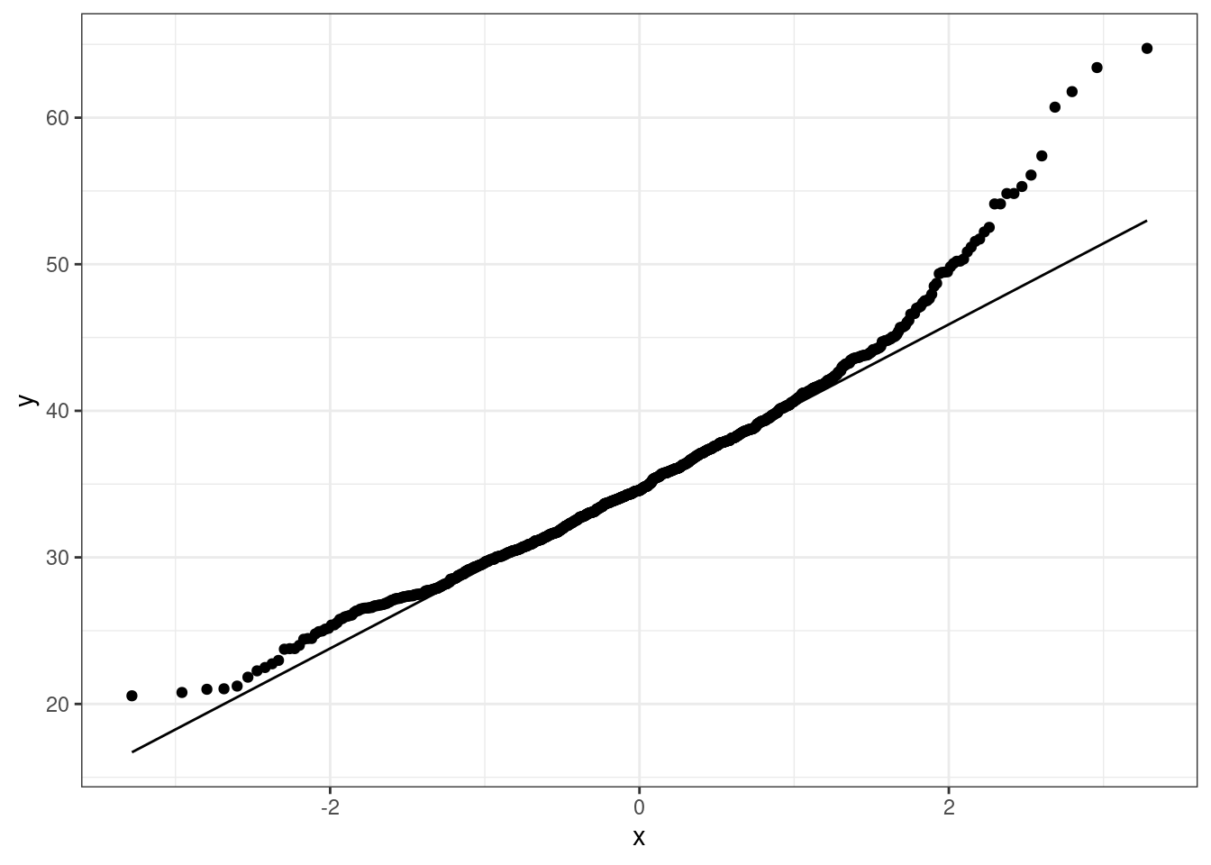
  theme_bw()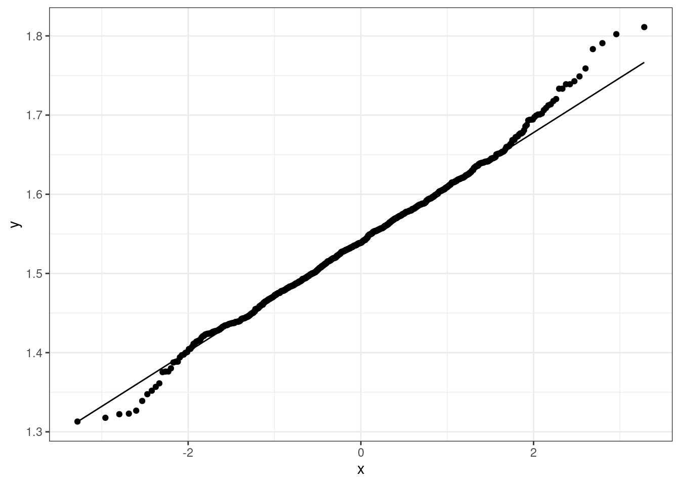

leicester_2011OAC_trans %>% 
  ggplot(aes(
    x = log10_u020
  )) +
  geom_histogram() +
  theme_bw()

## `stat_bin()` using `bins = 30`. Pick better value with `binwidth`.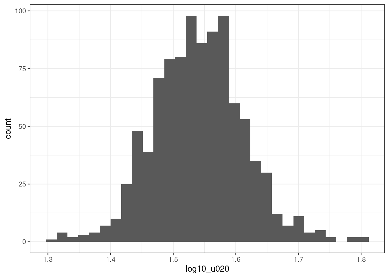

leicester_2011OAC_trans %>% 
  pull(log10_u020) %>% 
  shapiro.test()

## 
##  Shapiro-Wilk normality test
## 
## data:  .
## W = 0.99474, p-value = 0.001888

leicester_2011OAC_trans %>% 
  ggplot(aes(
    x = ihs_u020
  )) +
  geom_histogram() +
  theme_bw()

## `stat_bin()` using `bins = 30`. Pick better value with `binwidth`.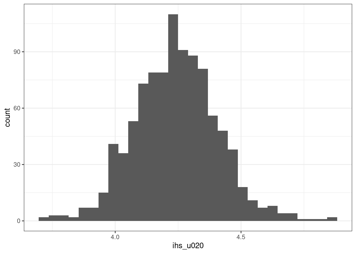

leicester_2011OAC_trans %>% 
  ggplot(aes(
    sample = ihs_u020
  )) +
  stat_qq() +
  stat_qq_line() +
  theme_bw()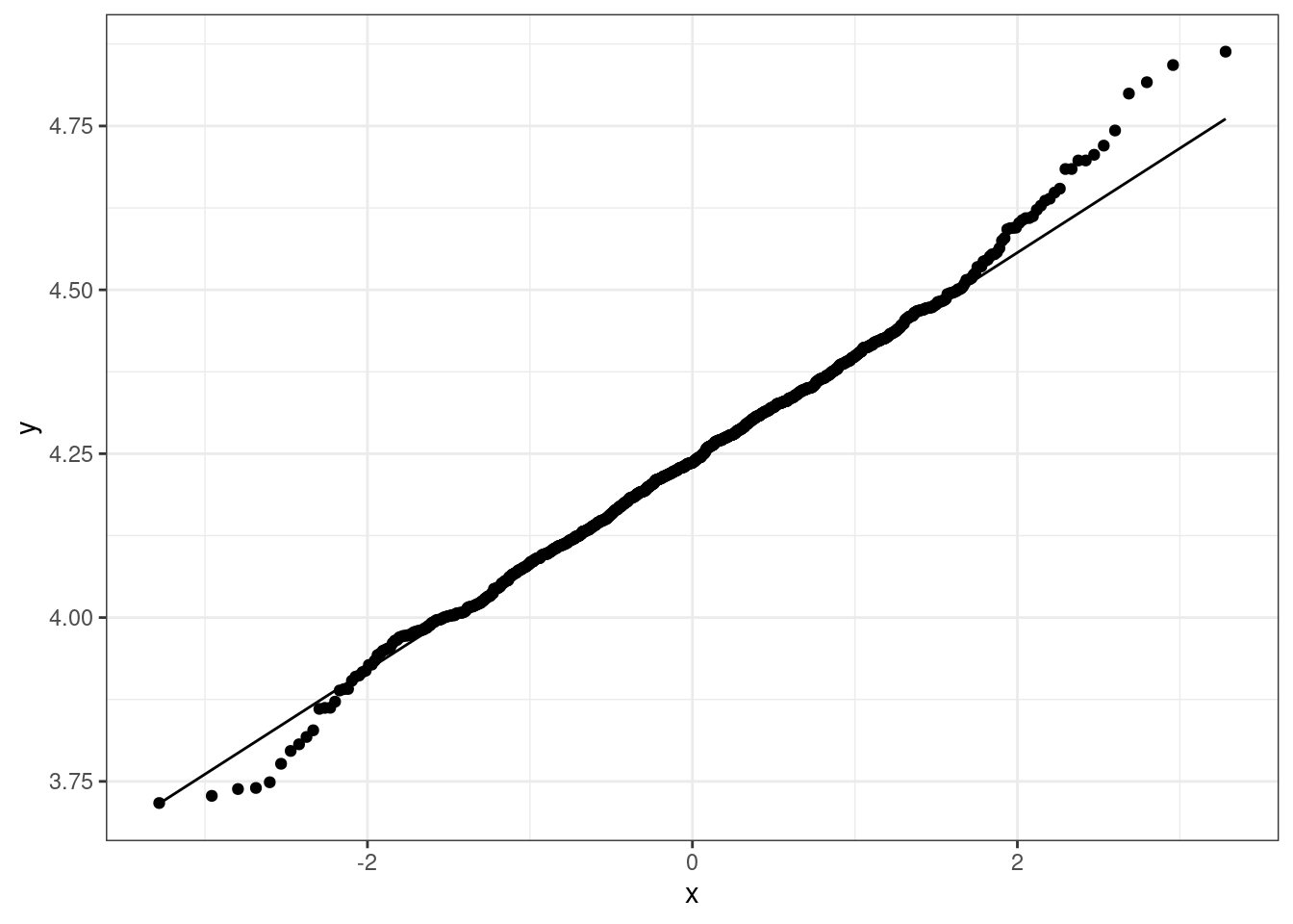

leicester_2011OAC_trans %>% 
  pull(ihs_u020) %>% 
  shapiro.test()

## 
##  Shapiro-Wilk normality test
## 
## data:  .
## W = 0.99473, p-value = 0.001874

Even using a logarithmic or inverse hyperbolic sine transformation, the variable u020 is still not normally distributed. The p-values are higher compared to the original variable, but still well below the \(0.01\) threshold. As visible in the charts, the transformed variables still show some level of long tails on both sides.

Question 203.1.2: Check whether the values of mean age (u020) are normally distributed when looking at the different 2011OAC supergroups separately. Check whether they can be transformed to a normally distributed set using logarithmic or inverse hyperbolic sine functions.

Note how the code below pivotes the table to obtain one column per 2011OAC supergroup.

leicester_2011OAC %>% 
  select(OA11CD, supgrpname, u020) %>% 
  pivot_wider(
    id_cols = OA11CD,
    names_from = supgrpname,
    names_prefix = "u020 ",
    values_from = u020
  ) %>% 
  select(-OA11CD) %>% 
  stat.desc(
    basic = FALSE,
    desc = FALSE,
    norm = TRUE
  ) %>% 
  kable(digits = 2)

	u020 Suburbanites	u020 Cosmopolitans	u020 Multicultural Metropolitans	u020 Ethnicity Central	u020 Constrained City Dwellers	u020 Hard-Pressed Living	u020 Urbanites
skewness	0.83	1.15	0.56	1.81	1.40	1.42	1.04
skew.2SE	1.27	2.17	2.76	2.87	1.78	2.96	1.74
kurtosis	1.24	1.54	0.64	6.13	1.74	2.77	3.56
kurt.2SE	0.97	1.47	1.58	4.92	1.14	2.91	3.04
normtest.W	0.96	0.91	0.98	0.87	0.86	0.89	0.92
normtest.p	0.07	0.00	0.00	0.00	0.00	0.00	0.00

leicester_2011OAC_trans %>% 
  select(OA11CD, supgrpname, log10_u020) %>% 
  pivot_wider(
    id_cols = OA11CD,
    names_from = supgrpname,
    names_prefix = "log10 u020 ",
    values_from = log10_u020
  ) %>% 
  select(-OA11CD) %>% 
  stat.desc(
    basic = FALSE,
    desc = FALSE,
    norm = TRUE
  ) %>% 
  kable(digits = 2)

	log10 u020 Suburbanites	log10 u020 Cosmopolitans	log10 u020 Multicultural Metropolitans	log10 u020 Ethnicity Central	log10 u020 Constrained City Dwellers	log10 u020 Hard-Pressed Living	log10 u020 Urbanites
skewness	0.46	0.51	0.14	0.88	0.94	0.81	0.21
skew.2SE	0.71	0.97	0.69	1.39	1.20	1.69	0.35
kurtosis	0.44	0.23	0.01	1.77	0.36	1.14	1.78
kurt.2SE	0.34	0.22	0.01	1.42	0.23	1.19	1.51
normtest.W	0.98	0.97	1.00	0.95	0.92	0.95	0.95
normtest.p	0.64	0.04	0.51	0.02	0.02	0.00	0.02

leicester_2011OAC_trans %>% 
  select(OA11CD, supgrpname, ihs_u020) %>% 
  pivot_wider(
    id_cols = OA11CD,
    names_from = supgrpname,
    names_prefix = "ihs u020 ",
    values_from = ihs_u020
  ) %>% 
  select(-OA11CD) %>% 
  stat.desc(
    basic = FALSE,
    desc = FALSE,
    norm = TRUE
  ) %>% 
  kable(digits = 2)

	ihs u020 Suburbanites	ihs u020 Cosmopolitans	ihs u020 Multicultural Metropolitans	ihs u020 Ethnicity Central	ihs u020 Constrained City Dwellers	ihs u020 Hard-Pressed Living	ihs u020 Urbanites
skewness	0.46	0.51	0.14	0.88	0.94	0.81	0.21
skew.2SE	0.71	0.97	0.69	1.39	1.20	1.69	0.36
kurtosis	0.44	0.23	0.01	1.78	0.36	1.14	1.78
kurt.2SE	0.34	0.22	0.01	1.43	0.23	1.19	1.51
normtest.W	0.98	0.97	1.00	0.95	0.92	0.95	0.95
normtest.p	0.64	0.04	0.51	0.02	0.02	0.00	0.02

While the original u020 variable is only normally distributed (using a \(0.01\) threshold) for the Suburbanites supergroup, the transformed variables are normally distributed for all supergroups except Hard-Pressed Living.

Question 203.1.3: Is the distribution of mean age (u020) different in different 2011OAC supergroups in Leicester?

We use the variable transformed using a logarithmic transformation (which is easier to interpret than an inverse hyperbolic sine) and excluding the Hard-Pressed Living supergroup, to ensure that all groups taken into account are normally distributed. We can then test that using ANOVA.

Let’s start with a boxplot, which can also be horizontal, if the nominal variable (categories) is provides for the y aesthetic and the continuous variable is provides for the x aesthetic. In the example below, that choice makes the 2011OAC supergroup names easier to read.

leicester_2011OAC_trans %>% 
  select(OA11CD, supgrpname, log10_u020) %>% 
  filter(supgrpname != "Hard-Pressed Living") %>% 
  ggplot(
    aes(
      x = log10_u020, 
      y = supgrpname
    )
  ) +
  geom_boxplot() +
  theme_bw()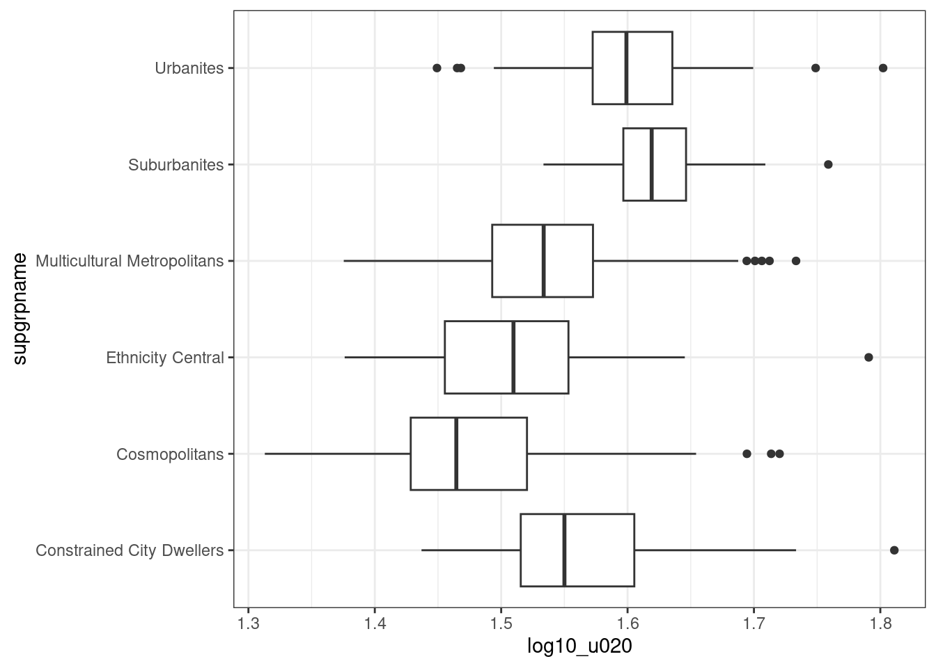

log10_u020_supgrpname_aov <-
  leicester_2011OAC_trans %>% 
  select(OA11CD, supgrpname, log10_u020) %>% 
  filter(supgrpname != "Hard-Pressed Living") %$% 
  aov(log10_u020 ~ supgrpname) %>%
  summary()

log10_u020_supgrpname_aov

##              Df Sum Sq Mean Sq F value Pr(>F)    
## supgrpname    5  1.049 0.20988   51.91 <2e-16 ***
## Residuals   862  3.485 0.00404                   
## ---
## Signif. codes:  0 '***' 0.001 '**' 0.01 '*' 0.05 '.' 0.1 ' ' 1

The test is significant F(5, 862) = 51.91 with p < .01, thus we can say that the distribution of u020 across the 2011OAC supergroups, excluding Hard-Pressed Living, are different.

Solutions 203.2

Question 203.2.1: As mentioned above, when discussing movement in cities, there is an assumption that people living in the city centre live in flats and work or cycle to work, whereas people living in the suburbs live in whole houses and commute via car. Study the correlation between the presence of flats (u089) and people commuting to work on foot, bicycle or other similar means (u122) in the same OAs. Consider whether the values might need to be normalised or otherwised transformed before starting the testing procedure.

The first necessary step is to normalise the data using the variable statistical unit Total_Household_Spaces for u089 and Total_Pop_No_NI_Students_16_to_74 for u122 as suggested by the lookup table.

flats_commuting <-
  leicester_2011OAC %>% 
  mutate(
    u089n = (u089 / Total_Household_Spaces) * 100,
    u122n = (u122 / Total_Pop_No_NI_Students_16_to_74) * 100
  ) %>% 
  select(OA11CD, u089n, u122n)

flats_commuting %>% 
  ggplot(aes(
    x = u089n
  )) +
  geom_histogram() +
  theme_bw()

## `stat_bin()` using `bins = 30`. Pick better value with `binwidth`.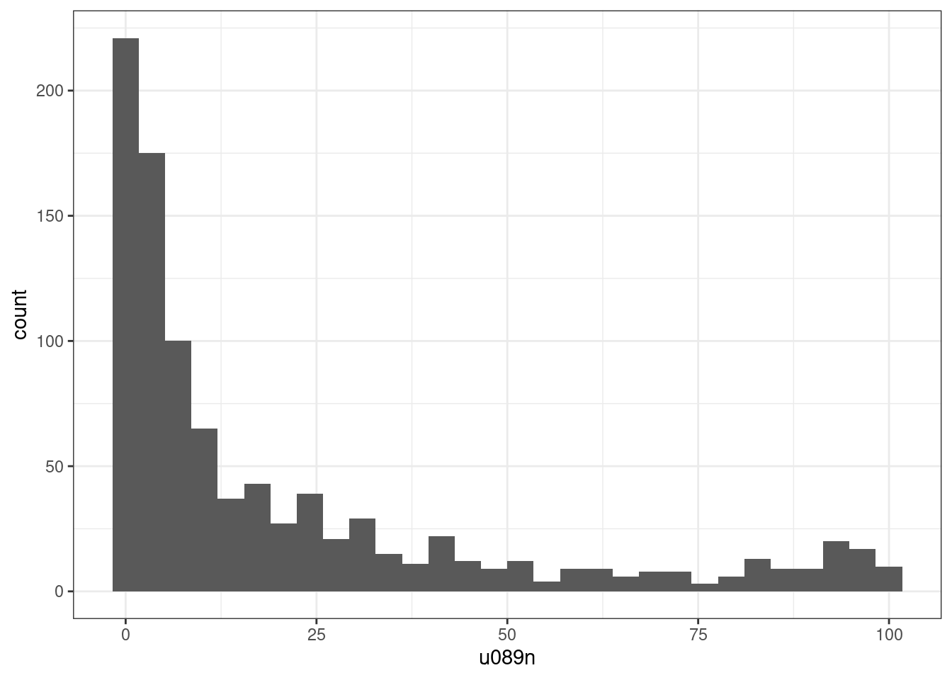

flats_commuting %>% 
  ggplot(aes(
    x = u122n
  )) +
  geom_histogram() +
  theme_bw()

## `stat_bin()` using `bins = 30`. Pick better value with `binwidth`.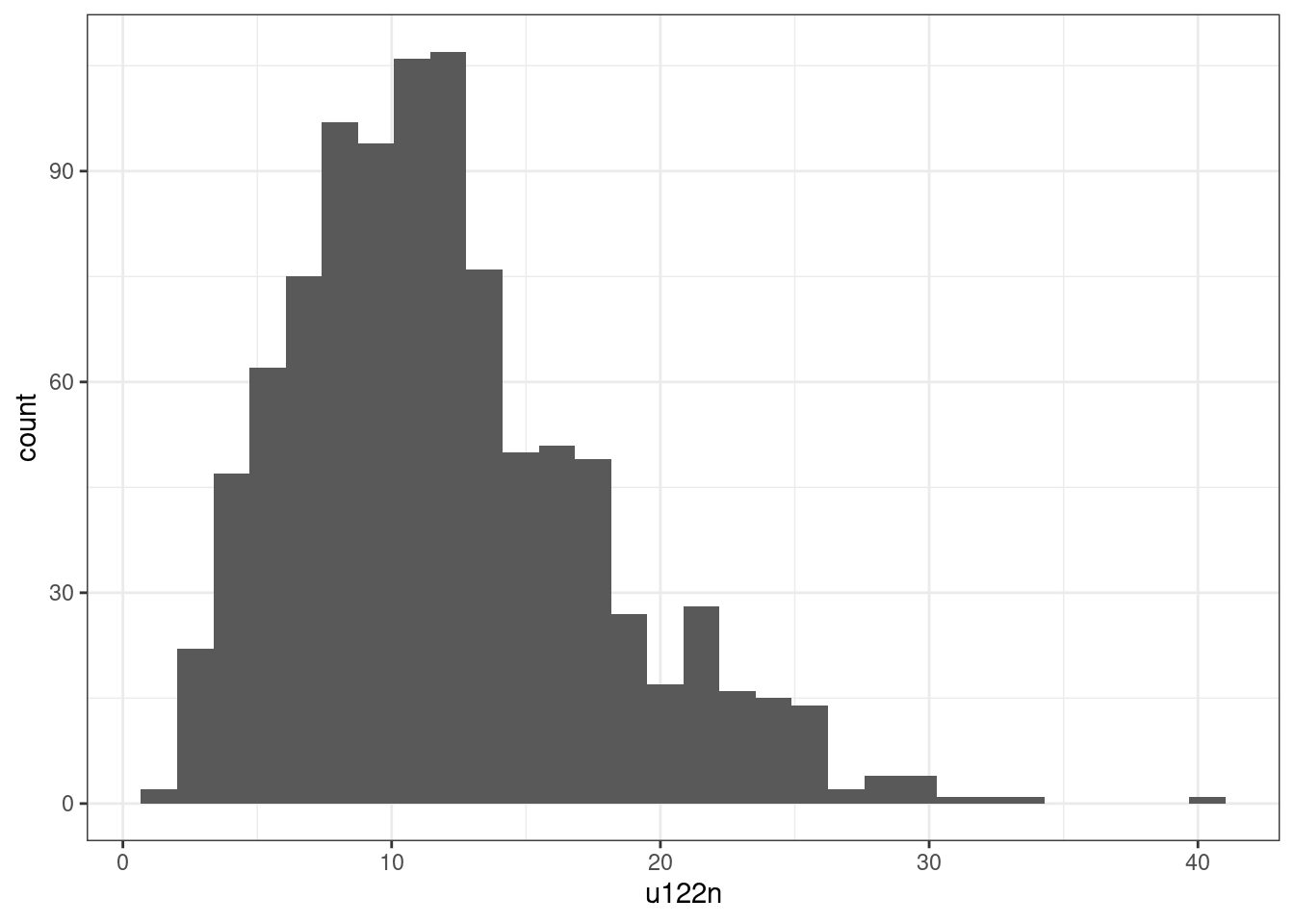

flats_commuting %>% 
  select(u089n, u122n) %>%
  stat.desc(
    basic = FALSE,
    desc = FALSE,
    norm = TRUE
  ) %>% 
  kable(digits = 2)

	u089n	u122n
skewness	1.56	0.85
skew.2SE	9.94	5.40
kurtosis	1.33	0.85
kurt.2SE	4.23	2.72
normtest.W	0.74	0.96
normtest.p	0.00	0.00

The two plots and the table above indicate that the two variables are not normally distributed and left skewed. As such, we can try to apply a logarithmic transformation to both to try to “un-skew” them. Note how rename_with uses a purrr-style lamba shorthand to to paste log10_ in front of all column names.

flats_commuting %>% 
  select(u089n, u122n) %>%
  mutate(
    across(
      everything(),
      log10
    )
  ) %>% 
  rename_with(
    # this is a shorthand
    # to paste log10_ in front
    # of all column names
    ~ paste0("log10_", .x)
  ) %>% 
  stat.desc(
    basic = FALSE,
    desc = FALSE,
    norm = TRUE
  ) %>% 
  kable(digits = 2)

	log10_u089n	log10_u122n
skewness	NaN	-0.59
skew.2SE	NaN	-3.73
kurtosis	NaN	0.63
kurt.2SE	NaN	2.01
normtest.W	NaN	0.98
normtest.p	NaN	0.00

The presence of NaN values in the u089 column indicates that the variable includes zeros, for which the logarithm is not defined. As such, we can try using the inverse iperbolic sine.

flats_commuting %>% 
  select(u089n, u122n) %>%
  mutate(
    across(
      everything(),
      asinh
    )
  ) %>% 
  rename_with(
    # this is a shorthand
    # to paste ihs_ in front
    # of all column names
    ~ paste0("ihs_", .x)
  ) %>% 
  stat.desc(
    basic = FALSE,
    desc = FALSE,
    norm = TRUE
  ) %>% 
  kable(digits = 2)

	ihs_u089n	ihs_u122n
skewness	-0.09	-0.53
skew.2SE	-0.59	-3.40
kurtosis	-1.10	0.43
kurt.2SE	-3.51	1.36
normtest.W	0.96	0.98
normtest.p	0.00	0.00

The values are now not NaN, but still, the variables are not normally distributed. As such, we can not use Pearson’s r correlation, as one of the assumptions is not met. In first instance, we can use Spearman’s rho to assess their correlation.

flats_commuting %>% 
  ggplot(aes(
    x = u089n,
    y = u122n
  )) +
  geom_point() +
  theme_bw()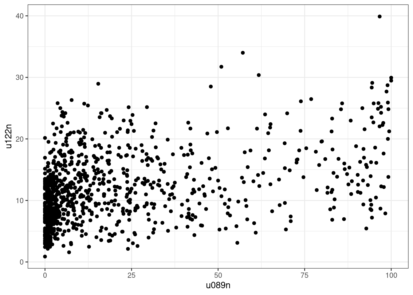

u089n_u122n_spearman <-
  flats_commuting %$%
  cor.test(
    u089n, u122n, 
    method = "spearman"
  )

## Warning in cor.test.default(u089n, u122n, method = "spearman"): Cannot compute
## exact p-value with ties

u089n_u122n_spearman

## 
##  Spearman's rank correlation rho
## 
## data:  u089n and u122n
## S = 92011434, p-value < 2.2e-16
## alternative hypothesis: true rho is not equal to 0
## sample estimates:
##       rho 
## 0.3932327

The output above includes the warning Warning: Cannot compute exact p-value with ties. As such, we need to check the number of ties in the dataset.

flats_commuting %>%
  count(u089n) %>%
  filter(n > 1) %>%
  count(wt = n()) %>%
  pull(n)

## Warning: `wt = n()` is deprecated
## ℹ You can now omit the `wt` argument

## [1] 127

flats_commuting %>%
  count(u122n) %>%
  filter(n > 1) %>%
  count(wt = n()) %>%
  pull(n)

## Warning: `wt = n()` is deprecated
## ℹ You can now omit the `wt` argument

## [1] 85

As the number of ties is sizable, the use of Kendall’s tau is advisable.

u089n_u122n_kendall <-
  flats_commuting %$%
  cor.test(
    u089n, u122n, 
    method = "kendall"
  )

u089n_u122n_kendall

## 
##  Kendall's rank correlation tau
## 
## data:  u089n and u122n
## z = 12.534, p-value < 2.2e-16
## alternative hypothesis: true tau is not equal to 0
## sample estimates:
##       tau 
## 0.2696906

The test is significant (p < .01), thus we can say that there is a relationship, which is however extremely weak. The value for tau is 0.27 indicating that the two variables share only 7.3% of variance.

Question 203.2.2: Another interesting issue to explore is the relationship between car ownership and the use of public transport. Study the correlation between the presence of households owning 2 or more cars or vans (u118) and people commuting to work via public transport (u120) or on foot, bicycle or other similar means (u122) in the same OAs. Consider whether the values might need to be normalised or otherwised transformed before starting the testing procedure.

The procedure is similar to the one seen above. The variable Total_Households should be used to normalise u118. Importantly, as the question specifies people commuting to work via public transport (u120) or on foot, bicycle or other similar means (u122) we also need to sum u120 and u122 to account for one or the other (as the answers in the census questions were mutually exclusive, only one mode could be chosen)

cas_vs_not_cars <-
  leicester_2011OAC %>% 
  mutate(
    u118n = (u118 / Total_Households) * 100,
    u120u122n = ((u120 + u122) / Total_Pop_No_NI_Students_16_to_74) * 100
  ) %>% 
  select(OA11CD, u118n, u120u122n)

cas_vs_not_cars %>% 
  ggplot(aes(
    x = u118n
  )) +
  geom_histogram() +
  theme_bw()

## `stat_bin()` using `bins = 30`. Pick better value with `binwidth`.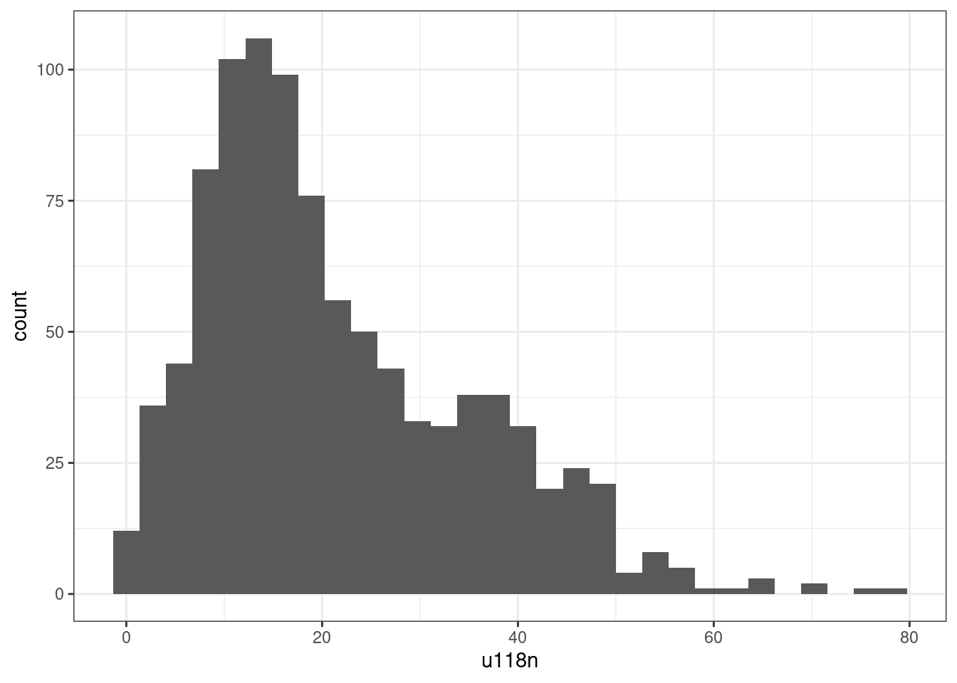

cas_vs_not_cars %>% 
  ggplot(aes(
    x = u120u122n
  )) +
  geom_histogram() +
  theme_bw()

## `stat_bin()` using `bins = 30`. Pick better value with `binwidth`.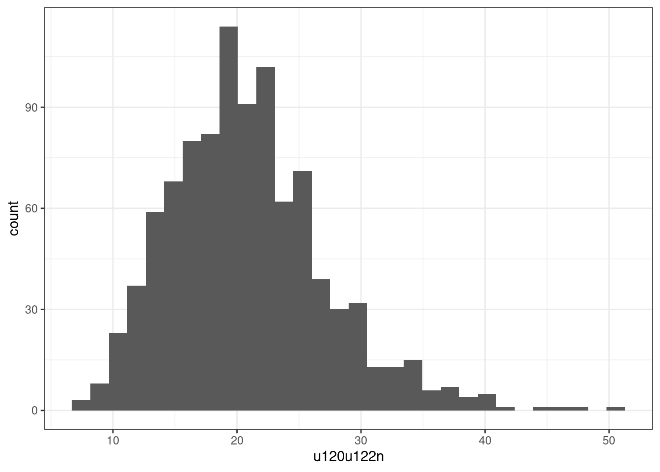

cas_vs_not_cars %>% 
  select(u118n, u120u122n) %>%
  stat.desc(
    basic = FALSE,
    desc = FALSE,
    norm = TRUE
  ) %>% 
  kable(digits = 2)

	u118n	u120u122n
skewness	0.91	0.79
skew.2SE	5.78	5.02
kurtosis	0.46	1.20
kurt.2SE	1.46	3.83
normtest.W	0.93	0.97
normtest.p	0.00	0.00

Again, both variables as not normally distributed. Thus, we can try to use a logarithmic transformation to try “un-skew” them.

cas_vs_not_cars %>% 
  select(u118n, u120u122n) %>%
  mutate(
    across(
      everything(),
      log10
    )
  ) %>% 
  rename_with(
    # this is a shorthand
    # to paste log10_ in front
    # of all column names
    ~ paste0("log10_", .x)
  ) %>% 
  stat.desc(
    basic = FALSE,
    desc = FALSE,
    norm = TRUE
  ) %>% 
  kable(digits = 2)

	log10_u118n	log10_u120u122n
skewness	NaN	-0.18
skew.2SE	NaN	-1.13
kurtosis	NaN	0.09
kurt.2SE	NaN	0.29
normtest.W	NaN	1.00
normtest.p	NaN	0.04

Again, u118n includes some zero value, thus producing NaN values in the table above. As such, we can try using the inverse hyperbolic sine.

cas_vs_not_cars %>% 
  select(u118n, u120u122n) %>%
  mutate(
    across(
      everything(),
      asinh
    )
  ) %>% 
  rename_with(
    # this is a shorthand
    # to paste ihs_ in front
    # of all column names
    ~ paste0("ihs_", .x)
  ) %>% 
  stat.desc(
    basic = FALSE,
    desc = FALSE,
    norm = TRUE
  ) %>% 
  kable(digits = 2)

	ihs_u118n	ihs_u120u122n
skewness	-0.95	-0.17
skew.2SE	-6.02	-1.11
kurtosis	1.70	0.09
kurt.2SE	5.41	0.28
normtest.W	0.95	1.00
normtest.p	0.00	0.04

Note how ihs_u120u122n is normally distributed, but ihs_u118n is not normally distributed. So, again we can’t use Pearson’s r correlation, and we resort to use Spearman’s rho.

cas_vs_not_cars %>% 
  ggplot(aes(
    x = u118n,
    y = u120u122n
  )) +
  geom_point() +
  theme_bw()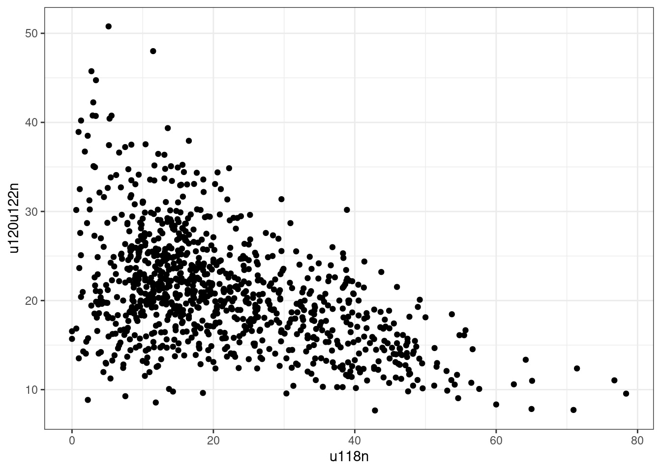

u118n_u120u122n_spearman <-
  cas_vs_not_cars %$%
  cor.test(
    u118n, u120u122n, 
    method = "spearman"
  )

## Warning in cor.test.default(u118n, u120u122n, method = "spearman"): Cannot
## compute exact p-value with ties

u118n_u120u122n_spearman

## 
##  Spearman's rank correlation rho
## 
## data:  u118n and u120u122n
## S = 217161157, p-value < 2.2e-16
## alternative hypothesis: true rho is not equal to 0
## sample estimates:
##        rho 
## -0.4320643

Note how the Spearman’s rho statistic is negative, indicating an inverse relationship between the to variables. That is a first indication that the more households with 2 or more cars or vans, the fewer people commute to work via public transport or on foot, bicycle or other similar means. However, again, the functions return the warning Warning: Cannot compute exact p-value with ties.

cas_vs_not_cars %>%
  count(u118n) %>%
  filter(n > 1) %>%
  count(wt = n()) %>%
  pull(n)

## Warning: `wt = n()` is deprecated
## ℹ You can now omit the `wt` argument

## [1] 115

cas_vs_not_cars %>%
  count(u120u122n) %>%
  filter(n > 1) %>%
  count(wt = n()) %>%
  pull(n)

## Warning: `wt = n()` is deprecated
## ℹ You can now omit the `wt` argument

## [1] 83

Again, the dataset contains a sizable number of ties, thus the use of Kendall’s tau is advisable.

u118n_u120u122n_kendall <-
  cas_vs_not_cars %$%
  cor.test(
    u118n, u120u122n, 
    method = "kendall"
  )

u118n_u120u122n_kendall

## 
##  Kendall's rank correlation tau
## 
## data:  u118n and u120u122n
## z = -14.278, p-value < 2.2e-16
## alternative hypothesis: true tau is not equal to 0
## sample estimates:
##        tau 
## -0.3065051

The test is significant (p < .01), thus we can say that there is an inverse relationship, which is however very weak. The value for tau is -0.307 indicating that the two variables share only 9.4% of variance.

Solutions 204

Solutions 204.1

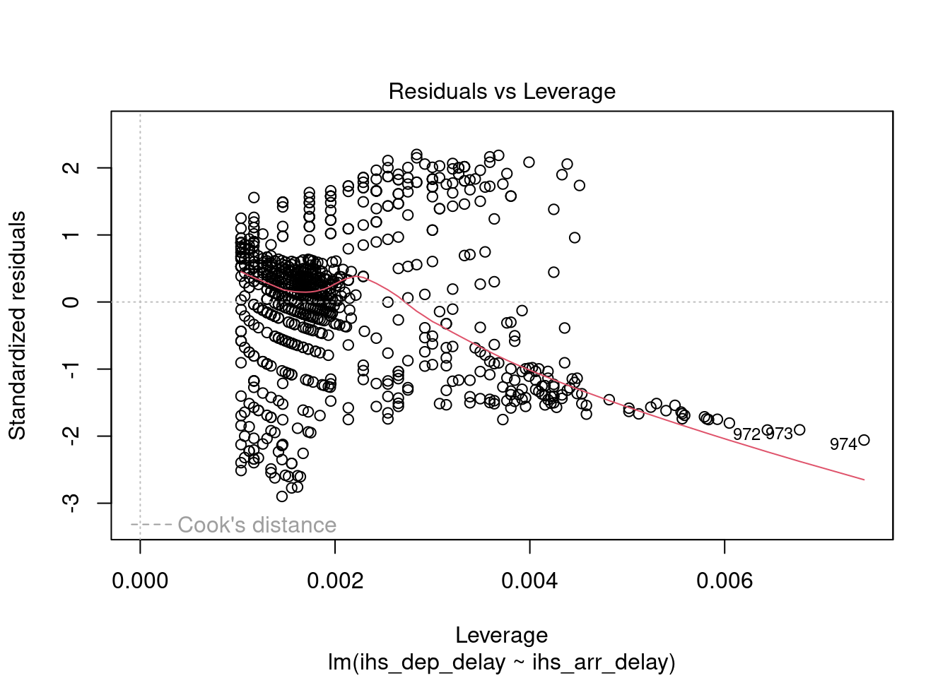
Question 204.1.1: While linear regression modelling does not require the variables to be normally distributed, very skewed variables such as dep_delay and arr_delay might be a significant obstacle to a robust model. Is it possible to build a robust model using “un-skewed” variables?

As both variables, we can use the inverse hyperbolic sine (asinh) to “un-skew” the variables. However, as illustrated by the plot below, that “expands” the area around the origin of the two axis to the point that the linear relationship might be lost.

flights_nov_20 %>%
  mutate(
    ihs_dep_delay = asinh(-dep_delay),
    ihs_arr_delay = asinh(-arr_delay)
  ) %>%
  ggplot(
    aes(
      x = ihs_dep_delay, 
      y = ihs_arr_delay
    )
  ) +
  geom_point() + 
  coord_fixed(ratio = 1) +
  theme_bw()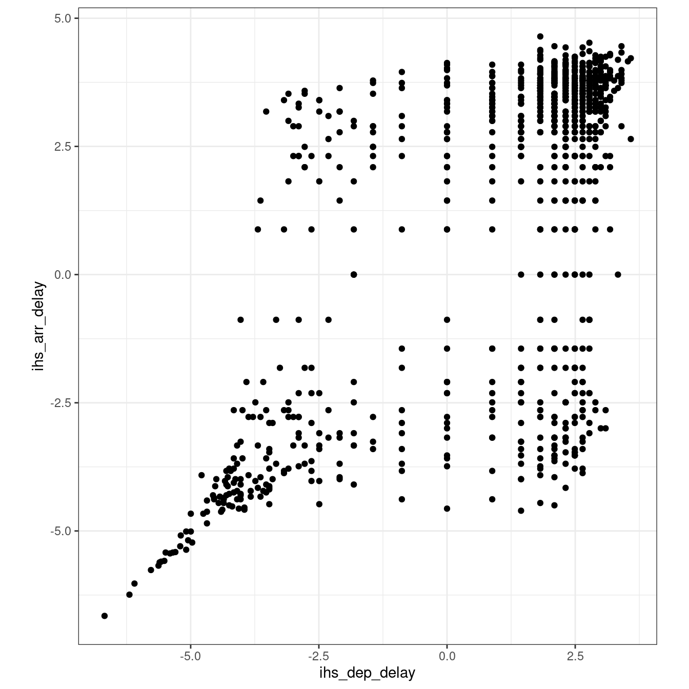

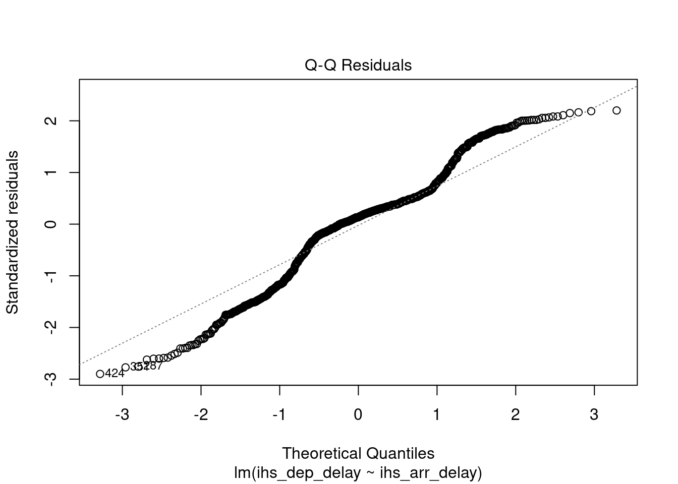
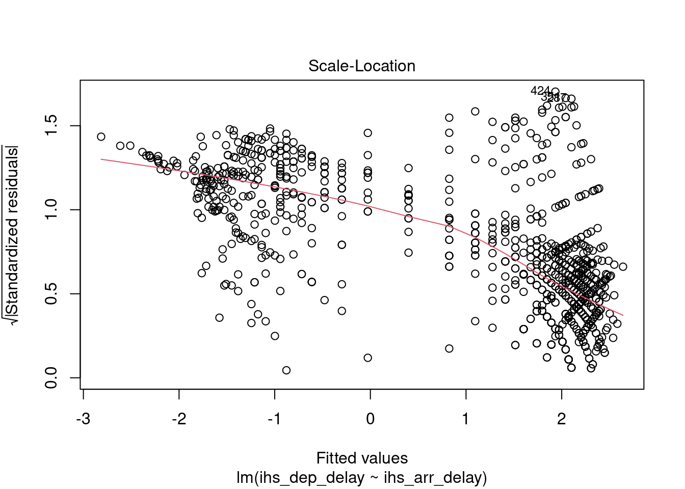
We can still try build a model. However, as illustrated below, the relaionship has become very weak, and the model is still not robust.

delay_model_2 <- flights_nov_20 %>% 
  mutate(
    ihs_dep_delay = asinh(-dep_delay),
    ihs_arr_delay = asinh(-arr_delay)
  ) %$%
  lm(ihs_dep_delay ~ ihs_arr_delay) 

delay_model_summary_2 <- delay_model_2 %>%
  summary()

delay_model_summary_2

## 
## Call:
## lm(formula = ihs_dep_delay ~ ihs_arr_delay)
## 
## Residuals:
##     Min      1Q  Median      3Q     Max 
## -5.4610 -1.0106  0.2507  0.9211  4.1417 
## 
## Coefficients:
##               Estimate Std. Error t value Pr(>|t|)    
## (Intercept)    0.39881    0.06441   6.192 8.75e-10 ***
## ihs_arr_delay  0.48274    0.01930  25.006  < 2e-16 ***
## ---
## Signif. codes:  0 '***' 0.001 '**' 0.01 '*' 0.05 '.' 0.1 ' ' 1
## 
## Residual standard error: 1.885 on 972 degrees of freedom
## Multiple R-squared:  0.3915, Adjusted R-squared:  0.3909 
## F-statistic: 625.3 on 1 and 972 DF,  p-value: < 2.2e-16

delay_model_2 %>% 
  rstandard() %>% 
  shapiro.test()

## 
##  Shapiro-Wilk normality test
## 
## data:  .
## W = 0.96798, p-value = 8.19e-14

delay_model_2 %>% 
  bptest()

## 
##  studentized Breusch-Pagan test
## 
## data:  .
## BP = 230.08, df = 1, p-value < 2.2e-16

delay_model_2 %>%
  dwtest()

## 
##  Durbin-Watson test
## 
## data:  .
## DW = 1.7535, p-value = 5.175e-05
## alternative hypothesis: true autocorrelation is greater than 0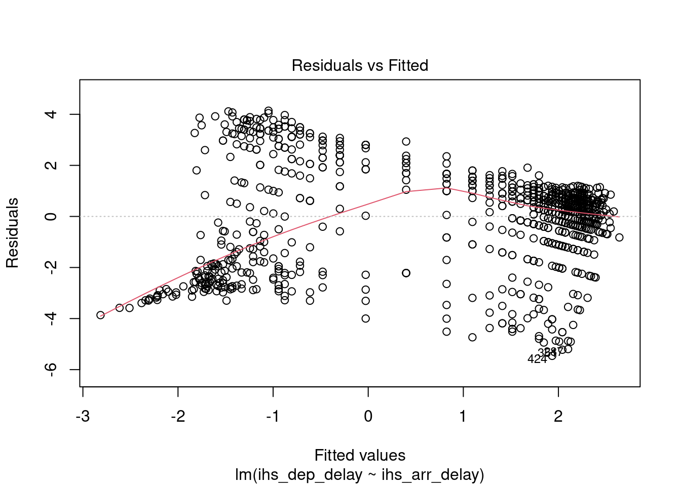

delay_model_2 %>% 
  plot()

An alternative approach might be to use a double square root function – i.e., square root of positive values and square root of the opposite of the value for negative values (more on if_else in the coming weeks). However, that seems not to fully resolve the issue.

flights_nov_20 %>%
  mutate(
    sqrt_dep_delay = 
      if_else(
        dep_delay >= 0, 
        sqrt(dep_delay), 
        (-1 * sqrt(-dep_delay)
      )
    ),
    sqrt_arr_delay = 
      if_else(
        arr_delay >= 0, 
        sqrt(arr_delay), 
        (-1 * sqrt(-arr_delay)
      )
    )
  ) %>%
  ggplot(
    aes(
      x = sqrt_dep_delay, 
      y = sqrt_arr_delay
    )
  ) +
  geom_point() + 
  coord_fixed(ratio = 1) +
  theme_bw()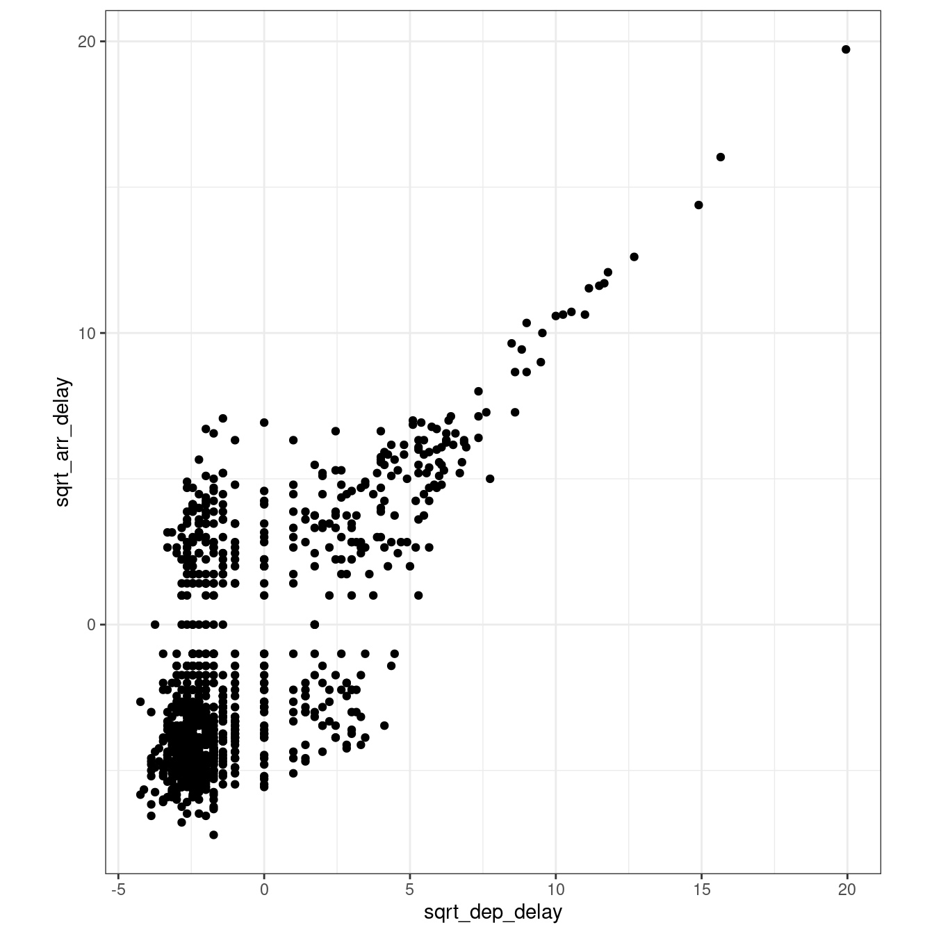

Solutions 204.2

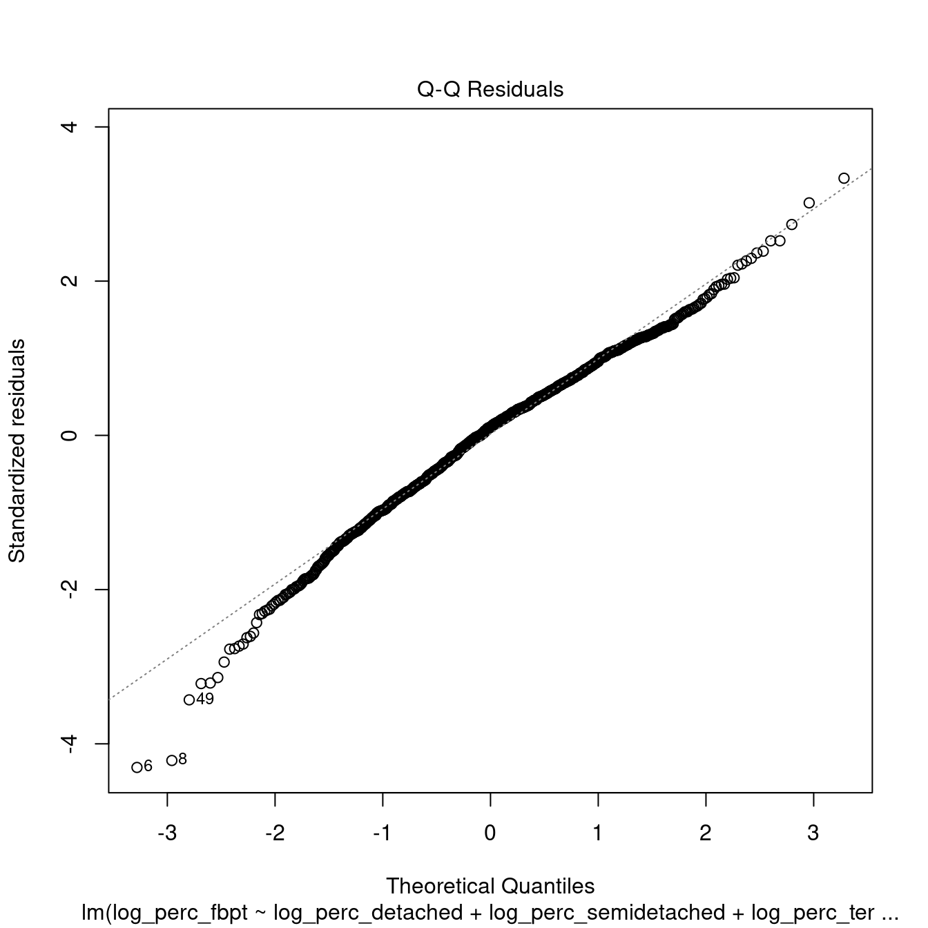
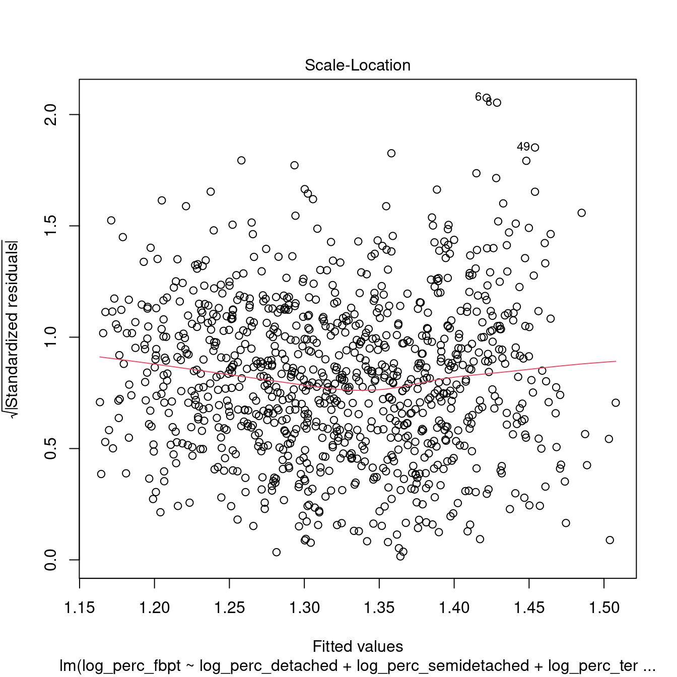
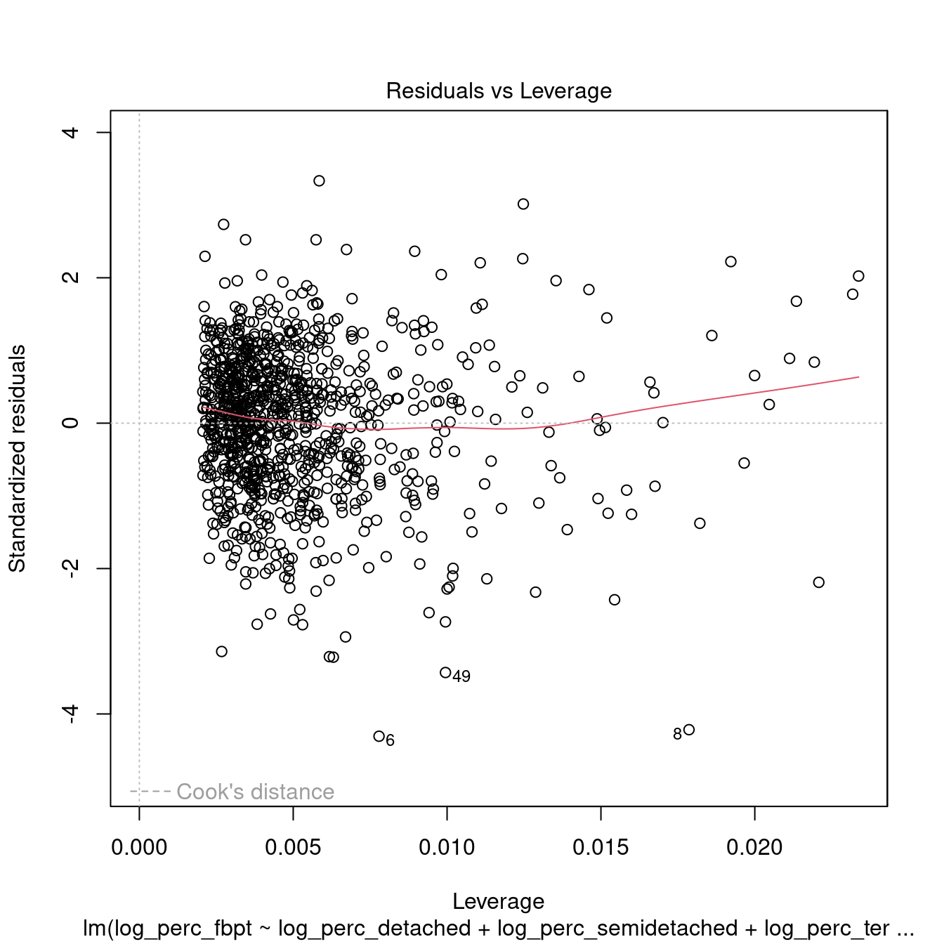
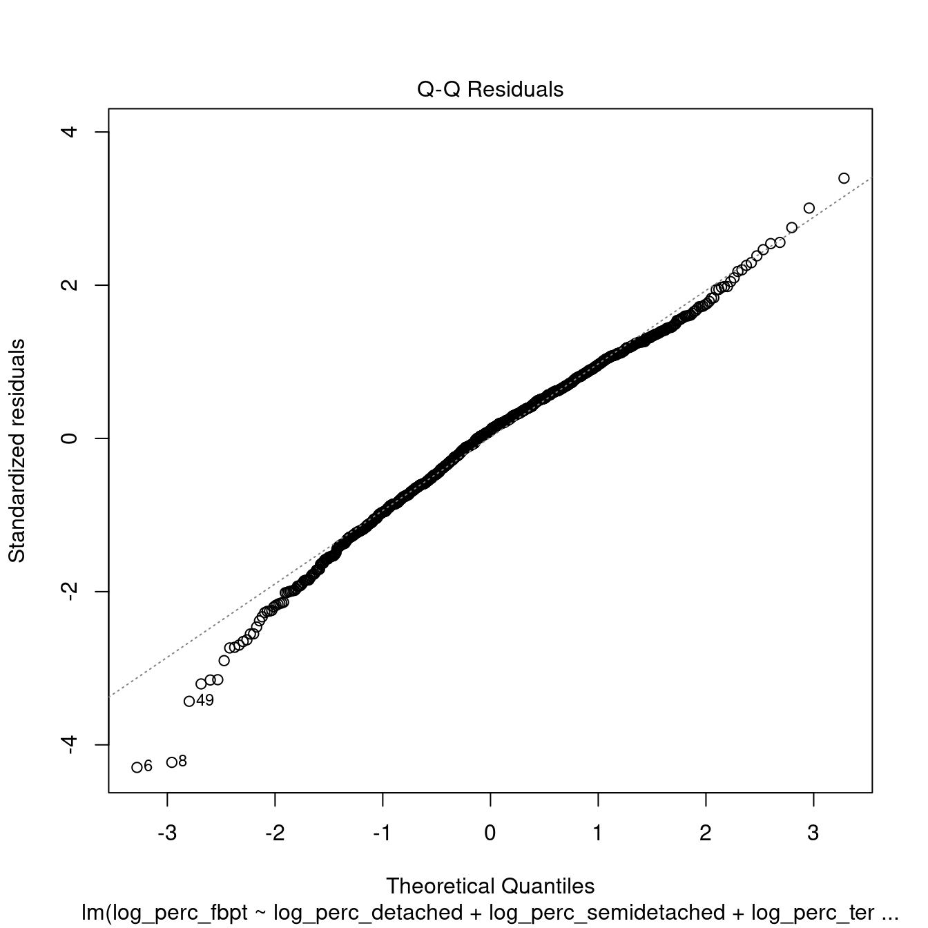
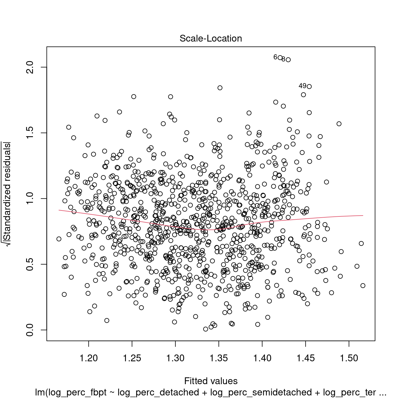
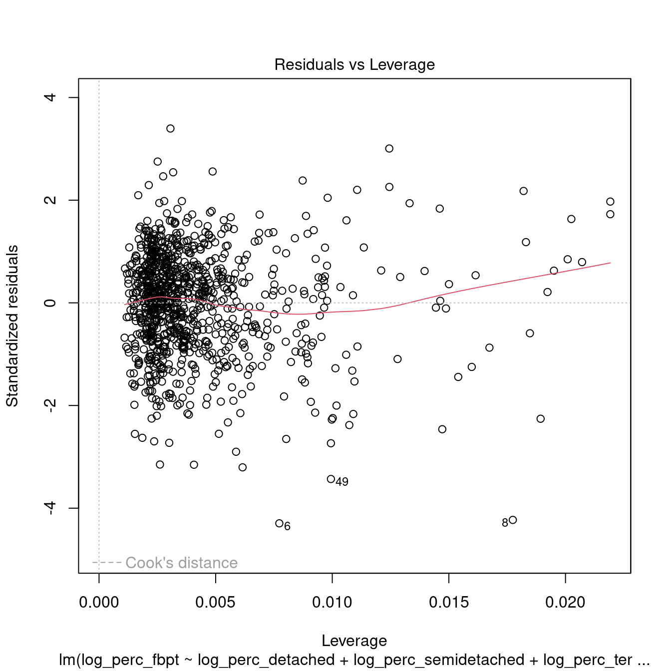
Question 204.2.1: Is it possible to create a model linking housing type (u086 to u090) to the number of people commuting to work via public transport (u120) or on foot, bicycle or other similar means (u122) in the same OAs?

There are five variables in the 2011OAC dataset related to housing type and two related to they type of commuting mentioned in the question (listed below). So, the first step is to extract and normalise those while also summing up the two variables related to commuting, as done in previous exercises.

u086: Whole house or bungalow: Detached
u087: Whole house or bungalow: Semi-detached
u088: Whole house or bungalow: Terraced (including end-terrace)
u089: Flats
u090: Caravan or other mobile or temporary structure
u120: Public Transport
u122: On foot, Bicycle or Other

leicester_dwellings <-
  leicester_2011OAC %>%
  dplyr::select(
    OA11CD, 
    Total_Dwellings, 
    Total_Pop_No_NI_Students_16_to_74,
    u120, u122,
    u086:u090
  ) %>%
  mutate(
    # On foot, Bicycle or Other
    # + Public Transport
    perc_fbpt = 
      ((u120 + u122) / 
         Total_Pop_No_NI_Students_16_to_74) * 100
  ) %>% 
  dplyr::mutate(
    dplyr::across( 
      u086:u090,
      #scale
      function(x){ (x / Total_Dwellings) * 100 }
    )
  ) %>%
  dplyr::rename(
    perc_detached = u086,
    perc_semidetached = u087,
    perc_terraced = u088,
    perc_flats = u089,   
    perc_carava_tmp = u090
  ) %>%
  # Remove columns not needed anymore
  select(
    -Total_Dwellings, 
    -Total_Pop_No_NI_Students_16_to_74,
    -u120, -u122
  ) %>% 
  arrange(perc_fbpt)

We can then explore the relationships between the variables using a pairs panel.

library(GGally)

leicester_dwellings %>%
  dplyr::select(perc_fbpt,perc_detached:perc_carava_tmp) %>%
  GGally::ggpairs(
    upper = list(continuous = wrap(ggally_cor, method = "kendall")),
    lower = list(continuous = wrap("points", alpha = 0.3, size=0.1))
  )

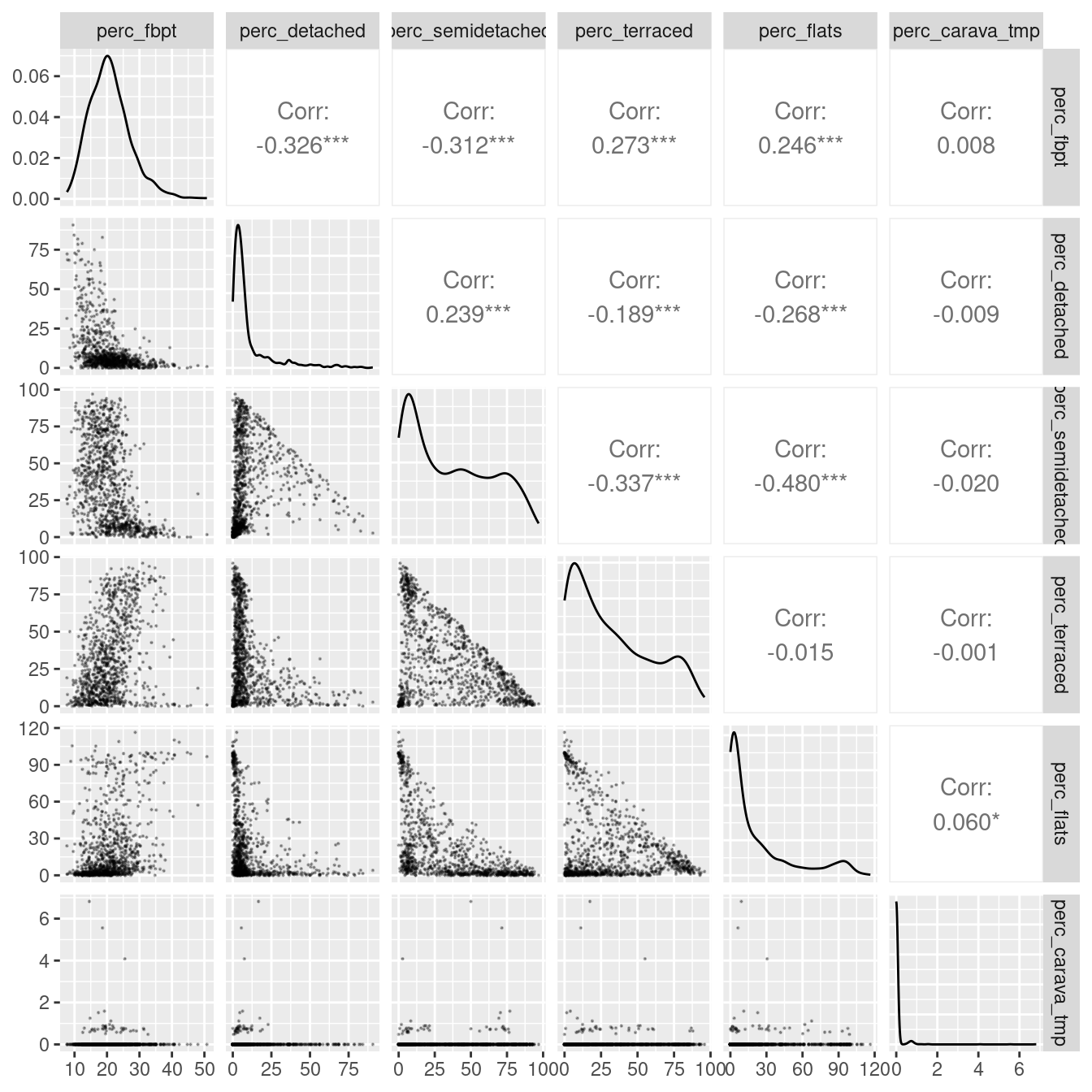
The plot above illustrates how the variable related to commuting via foot, bicycle or public transport in Leicester is very skewed. The same applies to the variables related to housing type. At the same time, the presence of Caravan or other mobile or temporary structure seems minimal. As such, we can attempt to remove the latter, and “un-skew” the rest using a logarithmic function. As there are cases in which at least one of the variables has minimum zero, we can take this example to explore the use of the function \(log_{10}(x+1)\) – which shift the logaritmic function to the left, so that the result is zero for \(x=0\).

leicester_dwellings %<>%
  dplyr::mutate(
    dplyr::across(
      c(perc_fbpt,perc_detached:perc_flats),
      ~ log10(.x + 1)
    )
  ) %>%
  dplyr::rename_with(
    ~ paste0("log_", .x),
    c(perc_fbpt,perc_detached:perc_flats)
  )

leicester_dwellings %>%
  dplyr::select(log_perc_fbpt,log_perc_detached:log_perc_flats) %>%
  GGally::ggpairs(
    upper = list(continuous = wrap(ggally_cor, method = "kendall")),
    lower = list(continuous = wrap("points", alpha = 0.3, size=0.1))
  )

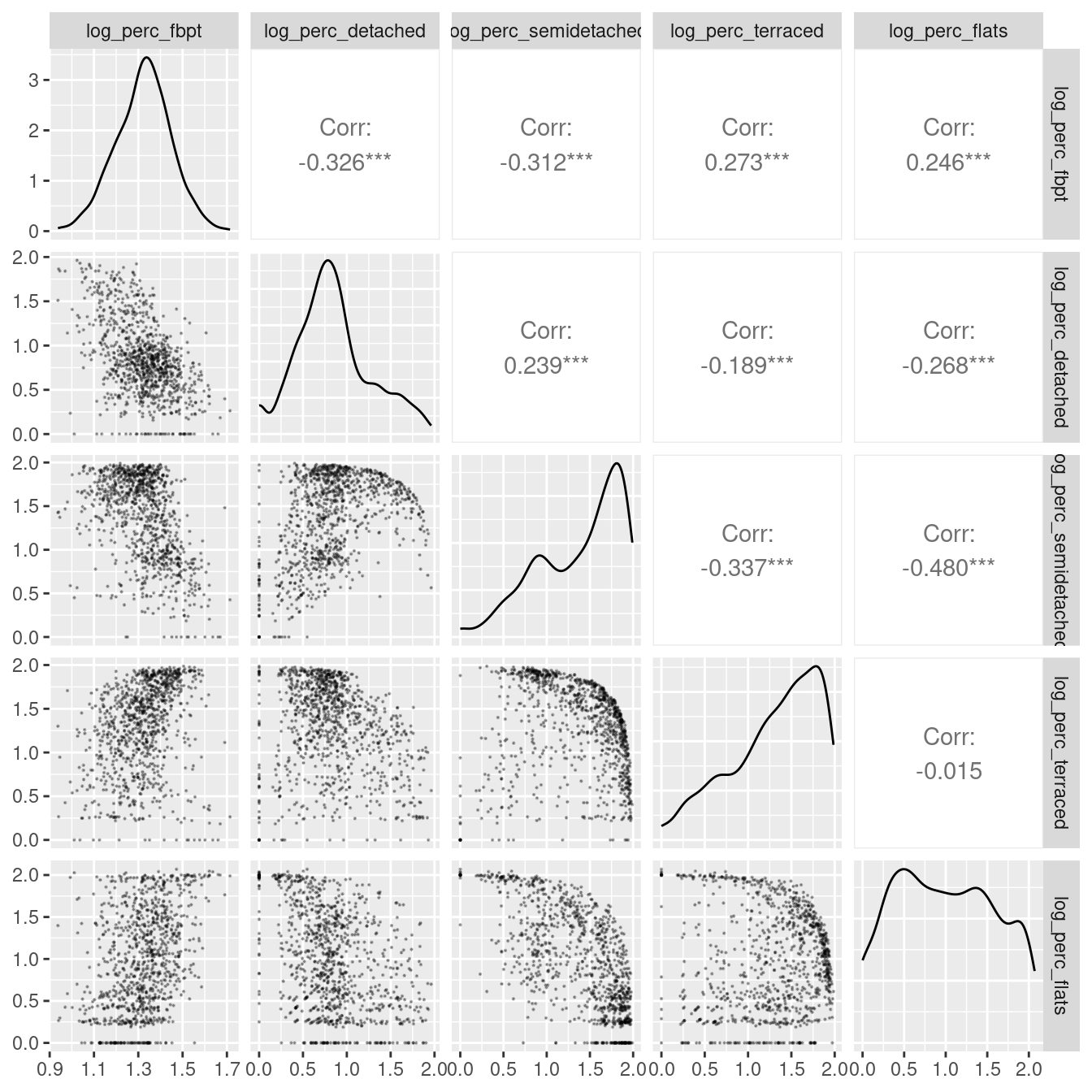
The plot above indicates a somewhat weak linear relationship between commuting via foot, bicycle or public transport and housing types. At the same time, there seems to be a clear relationship between semidetached houses and flats, which indicates a possible case of multicolinearity. Let’s try include all the variables above into a model and double-check multicolinearity.afterwards.

# Create model
dwellings_model1 <- 
  leicester_dwellings %$%
  lm(
    log_perc_fbpt ~ 
      log_perc_detached + log_perc_semidetached + 
      log_perc_terraced + log_perc_flats
  )

# Print summary
dwellings_model1 %>%
  summary()

## 
## Call:
## lm(formula = log_perc_fbpt ~ log_perc_detached + log_perc_semidetached + 
##     log_perc_terraced + log_perc_flats)
## 
## Residuals:
##      Min       1Q   Median       3Q      Max 
## -0.42849 -0.06348  0.01066  0.06716  0.33209 
## 
## Coefficients:
##                        Estimate Std. Error t value Pr(>|t|)    
## (Intercept)            1.441188   0.023965  60.136  < 2e-16 ***
## log_perc_detached     -0.097106   0.008704 -11.156  < 2e-16 ***
## log_perc_semidetached -0.071241   0.009176  -7.763 2.10e-14 ***
## log_perc_terraced      0.039661   0.006777   5.852 6.63e-09 ***
## log_perc_flats         0.009618   0.007510   1.281    0.201    
## ---
## Signif. codes:  0 '***' 0.001 '**' 0.01 '*' 0.05 '.' 0.1 ' ' 1
## 
## Residual standard error: 0.09989 on 964 degrees of freedom
## Multiple R-squared:  0.3602, Adjusted R-squared:  0.3576 
## F-statistic: 135.7 on 4 and 964 DF,  p-value: < 2.2e-16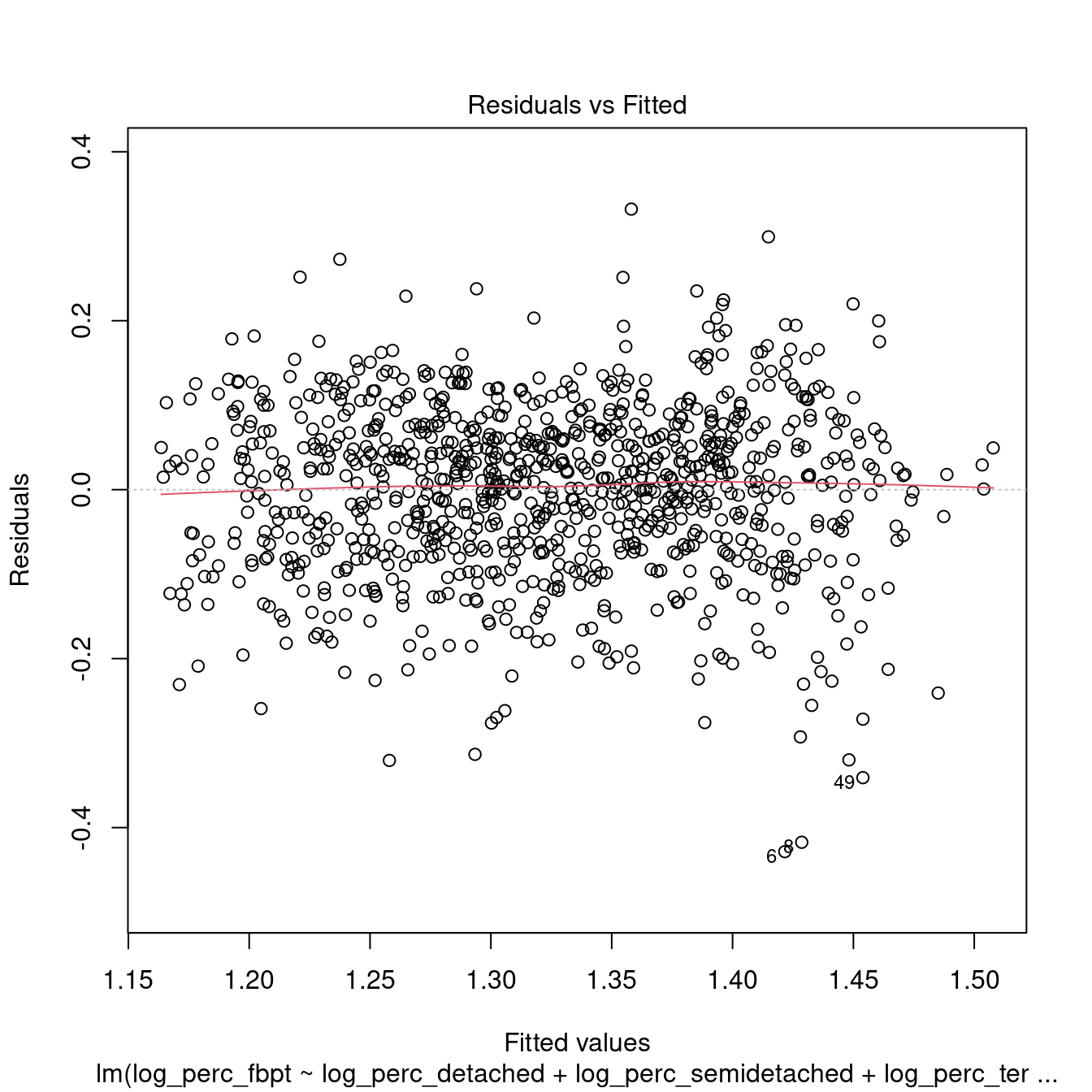

dwellings_model1 %>%
  plot()

dwellings_model1 %>%
  rstandard() %>% 
  shapiro.test()

## 
##  Shapiro-Wilk normality test
## 
## data:  .
## W = 0.98718, p-value = 1.722e-07

dwellings_model1 %>% 
  bptest()

## 
##  studentized Breusch-Pagan test
## 
## data:  .
## BP = 83.074, df = 4, p-value < 2.2e-16

dwellings_model1 %>%
  dwtest()

## 
##  Durbin-Watson test
## 
## data:  .
## DW = 0.71231, p-value < 2.2e-16
## alternative hypothesis: true autocorrelation is greater than 0

dwellings_model1 %>%
  vif()

##     log_perc_detached log_perc_semidetached     log_perc_terraced 
##              1.313314              1.948536              1.129558 
##        log_perc_flats 
##              1.943342

Interestingly, the results above don’t indicate a sigificant level or multicolinearity. However, the model is not robust. Also, we can see how the variable log_perc_flats is not significant in the model. Thus, we can try remove that variable and see whether there is any improvement.

# Create model
dwellings_model2 <- 
  leicester_dwellings %$%
  lm(
    log_perc_fbpt ~ 
      log_perc_detached + log_perc_semidetached + 
      log_perc_terraced
  )

# Print summary
dwellings_model2 %>%
  summary()

## 
## Call:
## lm(formula = log_perc_fbpt ~ log_perc_detached + log_perc_semidetached + 
##     log_perc_terraced)
## 
## Residuals:
##      Min       1Q   Median       3Q      Max 
## -0.42751 -0.06284  0.01012  0.06590  0.33884 
## 
## Coefficients:
##                        Estimate Std. Error t value Pr(>|t|)    
## (Intercept)            1.465339   0.014794  99.047  < 2e-16 ***
## log_perc_detached     -0.099686   0.008471 -11.768  < 2e-16 ***
## log_perc_semidetached -0.078462   0.007243 -10.833  < 2e-16 ***
## log_perc_terraced      0.037686   0.006601   5.709 1.51e-08 ***
## ---
## Signif. codes:  0 '***' 0.001 '**' 0.01 '*' 0.05 '.' 0.1 ' ' 1
## 
## Residual standard error: 0.09992 on 965 degrees of freedom
## Multiple R-squared:  0.3591, Adjusted R-squared:  0.3571 
## F-statistic: 180.3 on 3 and 965 DF,  p-value: < 2.2e-16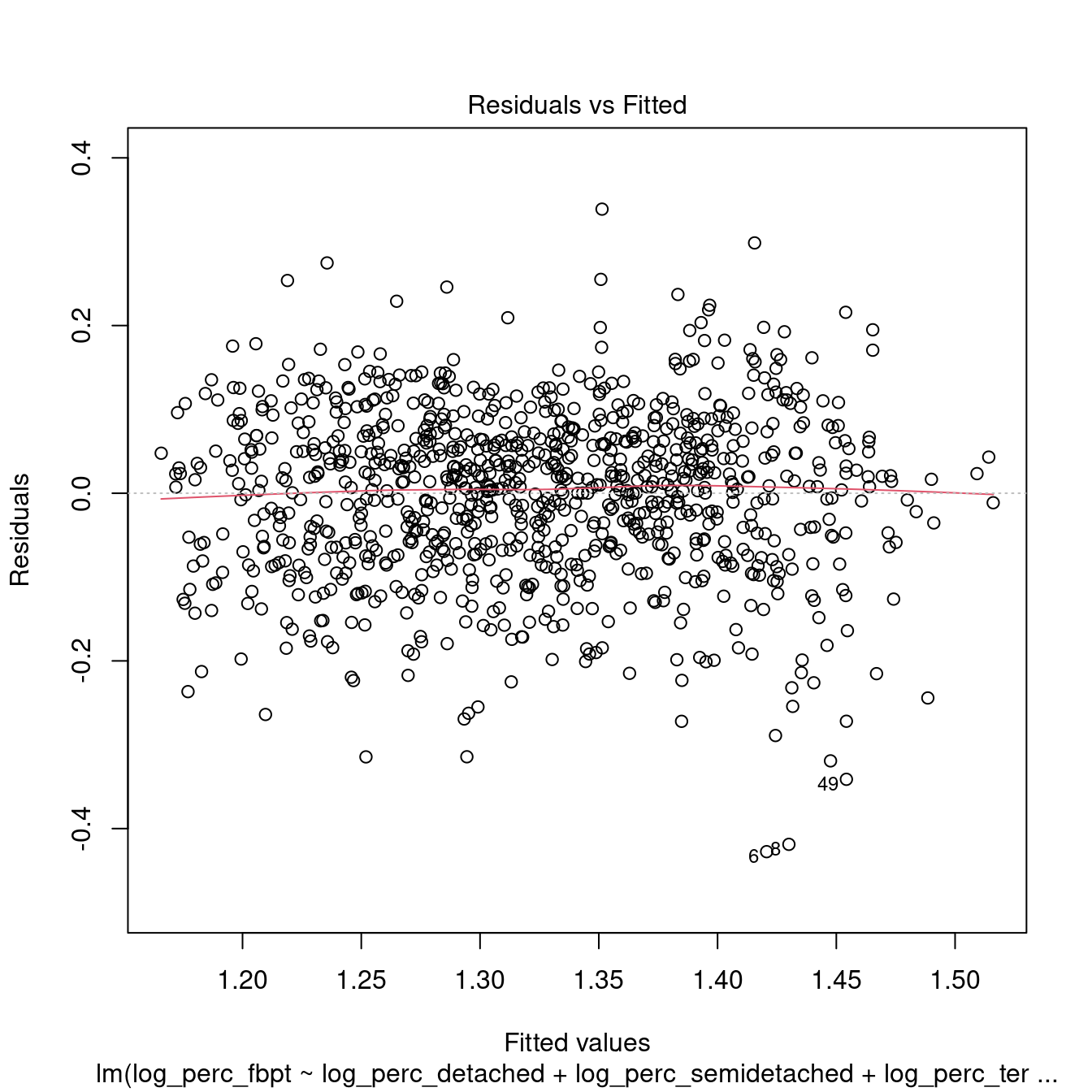

dwellings_model2 %>%
  plot()

dwellings_model2 %>%
  rstandard() %>% 
  shapiro.test()

## 
##  Shapiro-Wilk normality test
## 
## data:  .
## W = 0.98751, p-value = 2.413e-07

dwellings_model2 %>% 
  bptest()

## 
##  studentized Breusch-Pagan test
## 
## data:  .
## BP = 80.115, df = 3, p-value < 2.2e-16

dwellings_model2 %>%
  dwtest()

## 
##  Durbin-Watson test
## 
## data:  .
## DW = 0.71123, p-value < 2.2e-16
## alternative hypothesis: true autocorrelation is greater than 0

dwellings_model2 %>%
  vif()

##     log_perc_detached log_perc_semidetached     log_perc_terraced 
##              1.242958              1.212989              1.071107

All the variables within the models are now significant. However, the \(R^2\) is very low, indicating a very weak model. Moreover, the tests above indicate that the model is not robust.

Thus, we can conclude that, no, it seem like it is not possible to create a model linking population density to housing type in Leicester.

by Stefano De Sabbata – text licensed under the CC BY-SA 4.0, contains public sector information licensed under the Open Government Licence v3.0, code licensed under the GNU GPL v3.0.

Appendix 1

Groupwork exercise