12 R scripting

Print this chapter

12.1 Conditional statements

Conditional statements are fundamental in (procedural) programming, as they allow to execute or not execute part of a procedure depending on whether a certain condition is true. The condition is tested, and the part of the procedure to execute in the case the condition is true is included in a code block.

temperature <- 25

if (temperature > 25) {
  cat("It really warm today!")
}

A simple conditional statement can be created using if as in the example above. A more complex structure can be created using both if and else to provide not only a procedure to execute in case the condition is true but also an alternative procedure to be executed when the condition is false.

temperature <- 12

if (temperature > 25) {
  cat("It really warm today!")
} else {
  cat("Today is not warm")
}

## Today is not warm

Finally, conditional statements can be nested. That is, a conditional statement can be included as part of the code block to be executed after the condition is tested. For instance, in the example below, a second conditional statement is included in the code block to be executed in the case the condition is false.

temperature <- -5

if (temperature > 25) {
  cat("It really warm today!")
} else {
  if (temperature > 0) {
    cat("There is a nice temperature today")
  } else {
    cat("This is really cold!")
  }
}

## This is really cold!

Similarly, one of the examples seen in the lecture should be coded as follows.

a_value <- -7

if (a_value == 0) {
  cat("Zero")
} else {
  if (a_value < 0) {
    cat("Negative") 
  } else {
    cat("Positive")
  }
}

## Negative

Alternatively, the same set of conditions can be rewritten as follows.

a_value <- -7

if (a_value < 0) {
    cat("Negative") 
} else if (a_value == 0) {
  cat("Zero")
} else {
  cat("Positive")
}

## Negative

The choice of how to structure the conditions depends only on the logic behind the code that you are aiming to execute and the nature and order of the operations that need to be executed.

12.2 Loops

Loops are another core component of (procedural) programming and implement the idea of solving a problem or executing a task by performing the same set of steps a number of times. There are two main kinds of loops in R - deterministic and conditional loops. The former is executed a fixed number of times, specified at the beginning of the loop. The latter is executed until a specific condition is met. Both deterministic and conditional loops are extremely important in working with vectors.

12.2.1 Conditional Loops

In R, conditional loops can be implemented using while and repeat. The difference between the two is mostly syntactical: the first tests the condition first and then execute the related code block if the condition is true; the second executes the code block until a break command is given (usually through a conditional statement).

a_value <- 0
# Keep printing as long as x is smaller than 2
while (a_value < 2) {
  cat(a_value, "\n")
  a_value <- a_value + 1
}

## 0 
## 1

a_value <- 0
# Keep printing, if x is greater or equal than 2 than stop
repeat {
  cat(a_value, "\n")
  a_value <- a_value + 1
  if (a_value >= 2) break
}

## 0 
## 1

Conditional loops can be a source of issues within a script. If they are not accurately designed, they can enter into an infinite loop – for instance if the while condition is always TRUE or if the break condition within repeat always FALSE.

12.2.2 Deterministic Loops

The deterministic loop executes the subsequent code block iterating through the elements of a provided vector. During each iteration (i.e., execution of the code block), the current element of the vector is assigned to the variable in the statement, and it can be used in the code block.

It is, for instance, possible to iterate over a vector and print each of its elements.

east_midlands_cities <- c("Derby", "Leicester", "Lincoln", "Nottingham")

for (city in east_midlands_cities){
  cat(city, "\n")
}

## Derby 
## Leicester 
## Lincoln 
## Nottingham

It is common practice to create a vector of integers on the spot (e.g., using the : operator) to execute a certain sequence of steps a pre-defined number of times.

for (iterator in 1:3) {
  cat("Exectuion number", iterator, ":\n")
  cat("    Step1: Hi!\n")
  cat("    Step2: How is it going?\n")
}

## Exectuion number 1 :
##     Step1: Hi!
##     Step2: How is it going?
## Exectuion number 2 :
##     Step1: Hi!
##     Step2: How is it going?
## Exectuion number 3 :
##     Step1: Hi!
##     Step2: How is it going?

12.3 Example: multiple Shapiro–Wilk tests

As seen during the lecture, it is possible to use control structures to scale up your analysis and design the code in a way so that an analysis step is executed on different data. The code below is a variation on what seen in class, and it illustrates how to conduct a simple analysis of the normal distribution of different sections of the input data.

library(tidyverse)
library(magrittr)
library(knitr)

leicester_2011OAC <- read_csv("2011_OAC_Raw_uVariables_Leicester.csv")

The chunck below ises the option results = 'asis', which allows to interpret the output as Markdown code. That allows to translate the presence of ### near the supergroup name into a third-level heading in the output.

for (
  
  current_supgrp in
    # Extract the list of unique supergroup names
    leicester_2011OAC %>% 
      pull(supgrpname) %>% 
      unique()
  
  ) {
  
  # Print supergroup name
  cat("\n\n")
  cat(
    # Use a markdown heading
    # including some space above and blow it
    "###",
    current_supgrp,
    "\n\n"
  )
  
  # Run a Shapiro–Wilk test
  current_shapiro_test <-
    leicester_2011OAC %>% 
    filter(supgrpname == current_supgrp) %>% 
    pull(Total_Population) %>%
    shapiro.test()
  
  # Extract p value
  current_p_value <-
    current_shapiro_test %$% 
    p.value
  
  # Print whether the distribution
  # is significant or not
  if (current_p_value > 0.01){
    cat(
      "\n\n",
      "The total population",
      "of OA in Leicester",
      "in areas classified as",
      current_supgrp,
      "is normally distributed",
      "\n\n"
    )
  } else {
    cat(
      "\n\n",
      "The total population",
      "of OA in Leicester",
      "in areas classified as",
      current_supgrp,
      "is not normally distributed",
      "\n\n"
    )
  }
  
  # Create an histogram
  current_hist <-
    leicester_2011OAC %>% 
    filter(supgrpname == current_supgrp) %>% 
    ggplot(aes(
      x = Total_Population
    )) +
    geom_histogram() +
    ggtitle(current_supgrp) +
    theme_bw() 
  
  # Print the histogram
  print(current_hist)
  
  cat("\n\n")
  
}

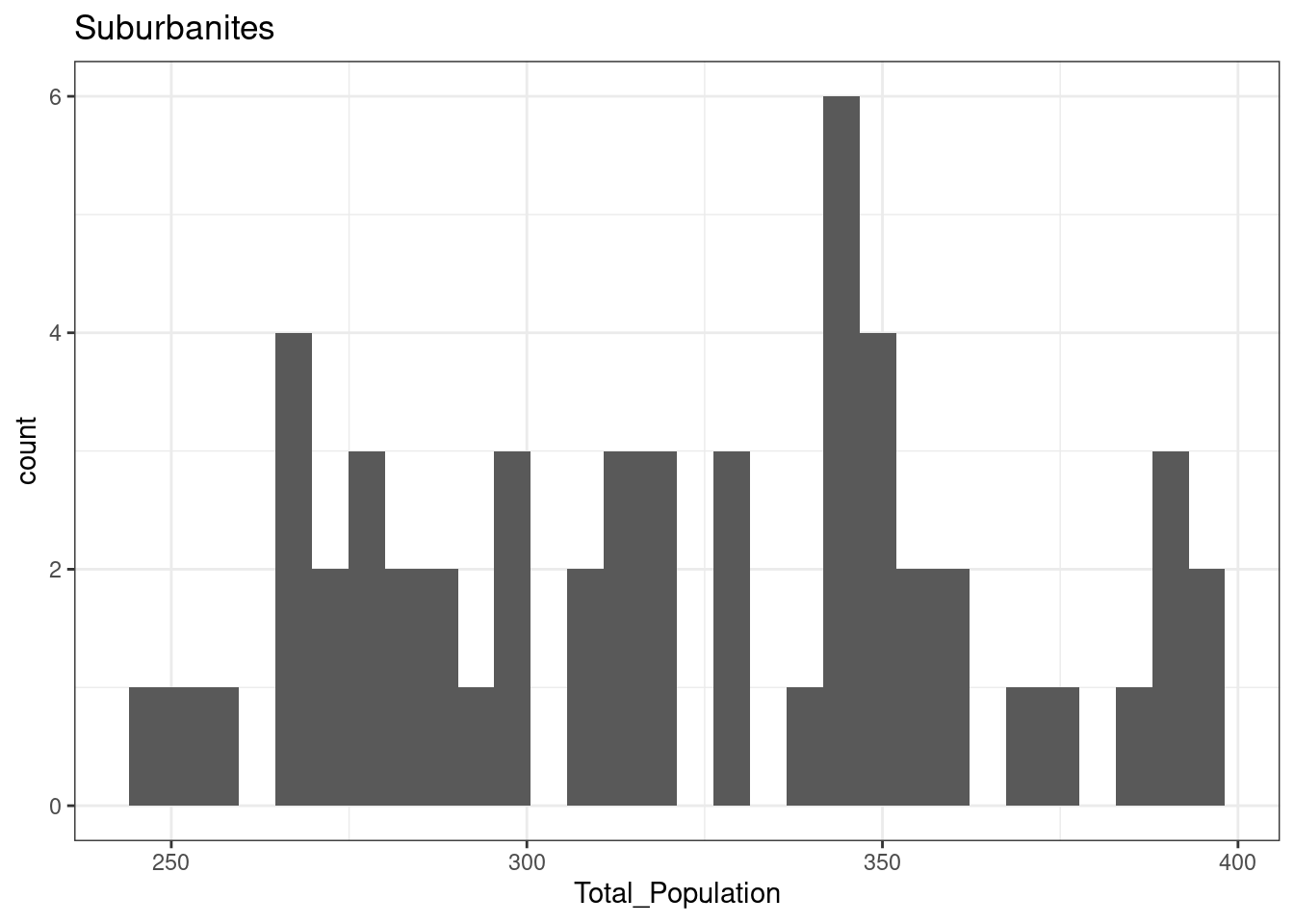
12.3.1 Suburbanites

The total population of OA in Leicester in areas classified as Suburbanites is normally distributed

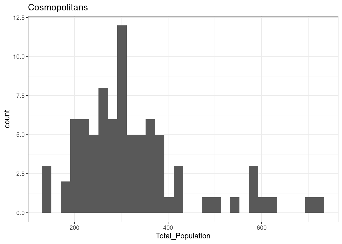
12.3.2 Cosmopolitans

The total population of OA in Leicester in areas classified as Cosmopolitans is not normally distributed

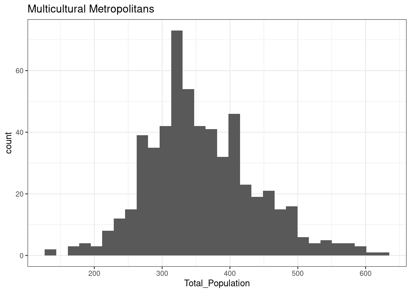
12.3.3 Multicultural Metropolitans

The total population of OA in Leicester in areas classified as Multicultural Metropolitans is not normally distributed

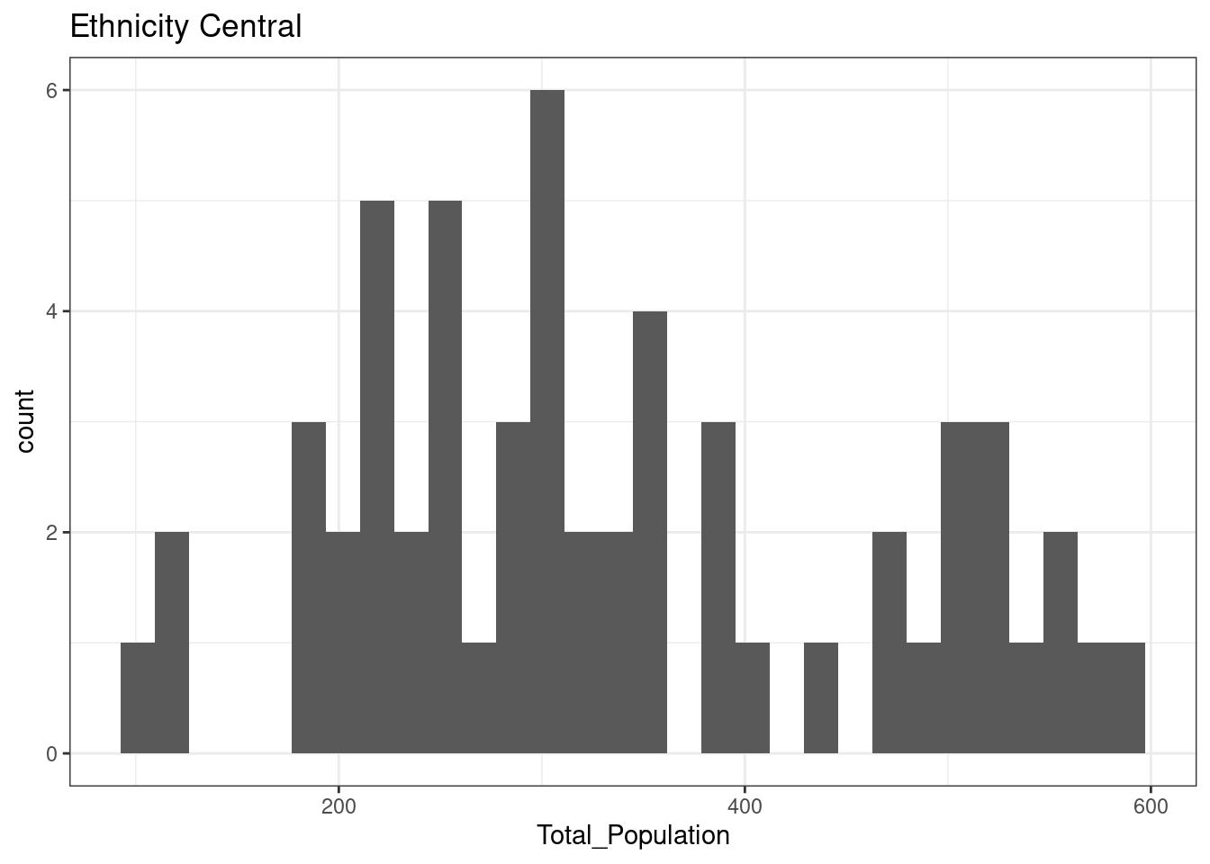
12.3.4 Ethnicity Central

The total population of OA in Leicester in areas classified as Ethnicity Central is normally distributed

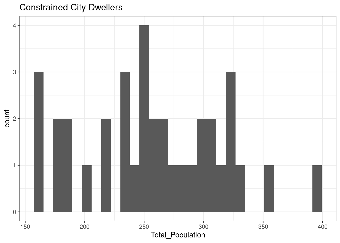
12.3.5 Constrained City Dwellers

The total population of OA in Leicester in areas classified as Constrained City Dwellers is normally distributed

12.3.6 Hard-Pressed Living

The total population of OA in Leicester in areas classified as Hard-Pressed Living is normally distributed

12.3.7 Urbanites

The total population of OA in Leicester in areas classified as Urbanites is normally distributed

12.4 Function definition

Recall from the first chapter that an algorithm or effective procedure is a mechanical rule, or automatic method, or programme for performing some mathematical operation (Cutland, 1980, p. 7²¹). A program is a specific set of instructions that implement an abstract algorithm. The definition of an algorithm (and thus a program) can consist of one or more functions, which are sets of instructions that perform a task, possibly using an input, possibly returning an output value.

The code below presents two versions of a simple function with one parameter. The function simply calculates the square root of a number and returns a value with two digits.

library(tidyverse)

sqrt_2digits <- 
  function (input_value) {
    sqrt_value <- sqrt(input_value)
    rounded_value <- round(sqrt_value, digits = 2)
    rounded_value
  }

sqrt_2digits_pipe <- 
  function (input_value) {
    input_value %>% 
      sqrt() %>% 
      round(digits = 2)
  }

Once the definition of a function has been executed, the function becomes part of the environment, and it should be visible in the Environment panel in a subsection titled Functions. Thereafter, the function can be called from the Console, from other portions of the script, as well as from other scripts.

sqrt_2digits(2)

## [1] 1.41

sqrt_2digits_pipe(2)

## [1] 1.41

12.4.1 Functions and control structures

One issue when writing functions is making sure that the data that has been given to the data is the right kind. For example, what happens when you try to compute the cube root of a negative number using a function as defined below?

cube_root <- function (input_value) {
   result <- input_value ^ (1 / 3)
   result
}

cube_root(-343)

## [1] NaN

That probably wasn’t the answer you wanted, as NaN (Not a Number) is the value returned when a mathematical expression is numerically indeterminate. In this case, this is actually due to a shortcoming with the ^ operator in R, which only works for positive base values. In fact \(-7\) is a perfectly valid cube root of \(-343\), since \((-7)\times(-7)\times(-7) = -343\).

To work around this limitation, we can state a conditional rule:

• If x < 0
  • calculate the cube root of x ‘normally’.
• Otherwise:
  • work out the cube root of the positive number, then change it to negative.

Those kinds of situations can be dealt with in an R function by using an if statement, as shown below. Note how the operator - (i.e., the symbol minus) is here used to obtain the inverse of a number, in the same way as -1 is the inverse of the number 1.

cube_root <- function (input_value) {
    if (input_value >= 0){
        result <- input_value^(1 / 3) 
    }else{
        result <- -( (-input_value)^(1/3) )
    }
    result
}

cube_root(343)
cube_root(-343)

However, other things can go wrong. For example, cube_root("Leicester") would cause an error to occur, Error in x^(1 / 3) : non-numeric argument to binary operator. That shouldn’t be surprising because cube roots only make sense for numbers, not character variables. Thus, it might be helpful if the cube root function could spot this and print a warning explaining the problem, rather than just crashing with a fairly cryptic error message such as the one above, as it does at the moment.

The function could be re-written to making use of is.numeric in a second conditional statement. If the input value is not numeric, the function returns the value NA (Not Available) instead of a number. Note that here there is an if statement inside another if statement, as it is always possible to nest code blocks – and if within a for within a while within an if within … etc.

cube_root <- function (input_value) { 
    if (is.numeric(input_value)) {
        if (input_value >= 0){
            result <- input_value^(1/3) 
        }else{
            result <- -(-input_value)^(1/3)
        }
        result
    }else{
        cat("WARNING: Input variable must be numeric\n") 
        NA
    }
}

Remember, cat is a printing function that instructs R to display the provided argument (in this case, the phrase within quotes) as output in the Console. The \n in cat tells R to add a newline when printing out the warning.

12.5 Debugging

The term bug is commonly used in computer science to refer to an error, failure, or fault in a system. The term `debugging'' in programming thus refers to the procedure of searching for mistakes in the code. This procedure can be simply done by re-reading and revising the written code, but R provides a useful command calleddebug`, that allows you to follow the execution of the code, and more easily identify mistakes.

Try debugging the function - since it is working properly, you won’t (hopefully!) find any errors, but that will demonstrate the debug facility, by typing debug(cube_root) in the RStudio Console. That tells R that you want to run cube_root in debug mode. Next enter cube_root(-50) in the RStudio Console and see how repeatedly pressing the return key steps you through the function. Note particularly what happens at the if statement.

At any stage in the process, you can type an R expression to check its value. For instance, when you get to the if statement, you can enter input_value > 0 in the RStudio Console to see whether it is true or false. Checking the value of expressions at various points when stepping through the code is a good way of identifying potential bugs or glitches in your code. Try running through the code for a few other cube root calculations, by replacing -50 above with different numbers, to get used to using the debugging facility.

When you are done, enter undebug(cube_root). That tells R that you are ready to return cube_root to running in normal mode. For further details about the debugger, enter help(debug) in the RStudio Console.

12.6 Writing functions for dplyr

The functions defined above are base R function, which not designed to work within the Tidyverse. Each one of the input is expected to be a number, although it can be applied to a vector. The functions are not designed to expect a dataframe or tibble as first argument (as Tidyverse functions such as select or mutate) and they are not designed to use the non-standard evaluation typical of the Tidyverse – i.e., when column names are provided as variable names, not as strings with quotes.

The Programming with dplyr article on the dplyr pages explains the process in full detail and it was the source of information for this section. To greatly simplify, to design functions for the Tidyverse, functions should expect the first argument to be a tibble (or dataframe). All the parameters that expect column names as argument using the non-standard evaluation need to be used while embracing them with doubled braces {{. Furthermore, in order to create output column names using the input column names the operator := must be used as illustrated below. Any additional paramenter can be provided as normal.

The example below defines a function named percentage_of, which calculates a new column which is the percentage of a column based on another column as total. The first parameter data expects a dataframe or tibbe as argument, while the two subsequent parameters expect column names to be used through non-standard evaluation. The function uses a mutate to add a new column. The new column is defined using the := operator and the name os perc_ followed by a column names, followed by _over_ and the name of the column used as total. The first and total columns are then used embraced with {{, dividing one by the other and finally multipled by a hundred.

percentage_of <- 
  function (data, var_col, total_col) {
    data %>%
      mutate(
        "perc_{{var_col}}" :=
          ({{ var_col }} / {{ total_col }}) * 100
      )
  }

The function can then be used to calculated the percentage of people in Leicester commuting to work using private transport (u121 in the 2011 Output Area Classification dataset seen in previous chapters), using the Total_Pop_No_NI_Students_16_to_74 as total. The first example below shows the procedure without the function. The second example shows the procedure using the function.

leicester_2011OAC <- read_csv("2011_OAC_Raw_uVariables_Leicester.csv")

library(knitr)

leicester_2011OAC %>%
  select(
    OA11CD, u121, Total_Pop_No_NI_Students_16_to_74
  ) %>%
  mutate(
    perc_u121 = 
      (u121 / Total_Pop_No_NI_Students_16_to_74) * 100
  ) %>%
  slice_head(n = 5) %>% 
  kable()

OA11CD	u121	Total_Pop_No_NI_Students_16_to_74	perc_u121
E00069517	113	225	50.22222
E00069514	102	287	35.54007
E00169516	94	282	33.33333
E00169048	111	227	48.89868
E00169044	110	231	47.61905

leicester_2011OAC %>%
  select(
    OA11CD, u121, Total_Pop_No_NI_Students_16_to_74
  ) %>%
  percentage_of(
    u121, Total_Pop_No_NI_Students_16_to_74
  ) %>%
  slice_head(n = 5) %>% 
  kable()

OA11CD	u121	Total_Pop_No_NI_Students_16_to_74	perc_u121
E00069517	113	225	50.22222
E00069514	102	287	35.54007
E00169516	94	282	33.33333
E00169048	111	227	48.89868
E00169044	110	231	47.61905

12.7 Loading R scripts

A key reason for writing functions is that you can write them once and they use them any time you need them. That is the principle behind the creation of libraries, which are (mostly) collections of functions. To that purpose, it is possible to write functions in an R script and then load that script (and all functions there defined) fromanother script or RMarkdown document – in a fashion similar to when a library is loaded. Create a new R script named my_useful_functions.R (as seen in this section), copy the code below in that R script and save the file.

library(tidyverse)

percentage_of <- 
  function (data, var_col, total_col) {
    data %>%
      mutate(
        "perc_{{var_col}}" :=
          ({{ var_col }} / {{ total_col }}) * 100
      )
  }

Create a new RMarkdown document and copy-paste the code below in the new document.

library(tidyverse)

source("my_useful_functions.R")

leicester_2011OAC <- read_csv("2011_OAC_Raw_uVariables_Leicester.csv")

leicester_2011OAC %>%
  select(
    OA11CD, u121, Total_Pop_No_NI_Students_16_to_74
  ) %>%
  percentage_of(
    u121, Total_Pop_No_NI_Students_16_to_74
  ) %>%
  slice_head(n = 5) %>% 
  kable()

When knitted, the new document uses source to instruct the interpreter load and run the code in my_useful_functions.R script, thus loading the definition of the percentage_of function. The rest of the code then load the 2011 OAC data and invokes the function within the pipe. That is a simple example, but this can be an extremely powerful tool to create your own library of functions to be used by different scripts.

---

by Stefano De Sabbata – text licensed under the CC BY-SA 4.0, contains public sector information licensed under the Open Government Licence v3.0, code licensed under the GNU GPL v3.0.