4 Table operations
The first two sections illustrate the pivot and join functionalities of the Tidyverse libraries using simple examples. The last section instead presents a more complex example, loading and wrangling with data related to the 2011 Output Area Classification and the Indexes of Multiple Deprivation 2015.
4.1 Long and wide table formats
Tabular data are usually presented in two different formats.
- Wide: this is the most common approach, where each real-world entity (e.g. a city) is represented by one single row and its attributes are represented through different columns (e.g., a column representing the total population in the area, another column representing the size of the area, etc.).
| City | Population | Area | Density |
|---|---|---|---|
| Leicester | 329,839 | 73.3 | 4,500 |
| Nottingham | 321,500 | 74.6 | 4,412 |
- Long: this is probably a less common approach, but still necessary in many cases, where each real-world entity (e.g. a city) is represented by multiple rows, each one reporting only one of its attributes. In this case, one column is used to indicate which attribute each row represent, and another column is used to report the value.
| City | Attribute | Value |
|---|---|---|
| Leicester | Population | 329,839 |
| Leicester | Area | 73.3 |
| Leicester | Density | 4,500 |
| Nottingham | Population | 321,500 |
| Nottingham | Area | 74.6 |
| Nottingham | Density | 4,412 |
The tidyr library provides two functions that allow transforming wide-formatted data to a long format, and vice-versa. Please take your time to understand the example below and check out the tidyr help pages before continuing.
city_info_wide <- data.frame(
    city = c("Leicester", "Nottingham"),
    population = c(329839, 321500),
    area = c(73.3, 74.6),
    density = c(4500, 4412)
  ) %>%
  as_tibble()

city_info_wide %>%
kable()| city | population | area | density |
|---|---|---|---|
| Leicester | 329839 | 73.3 | 4500 |
| Nottingham | 321500 | 74.6 | 4412 |
city_info_long <- city_info_wide %>%
  pivot_longer(
    # exclude IDs (city names) from the pivoted columns
    cols = -city,
    # name for the new column containing
    # the names of the old columns
    names_to = "attribute",
    # name for the new column containing
    # the values included under the old columns
    values_to = "value"
  )

city_info_long %>%
kable()| city | attribute | value |
|---|---|---|
| Leicester | population | 329839.0 |
| Leicester | area | 73.3 |
| Leicester | density | 4500.0 |
| Nottingham | population | 321500.0 |
| Nottingham | area | 74.6 |
| Nottingham | density | 4412.0 |
city_info_back_to_wide <- city_info_long %>%
  pivot_wider(
    # column containing the attribute names
    names_from = attribute,
    # column containing the values
    values_from = value
  )

city_info_back_to_wide %>%
kable()| city | population | area | density |
|---|---|---|---|
| Leicester | 329839 | 73.3 | 4500 |
| Nottingham | 321500 | 74.6 | 4412 |
4.2 Joining tables
A join operation combines two tables into one by matching rows that have the same values in the specified column. This operation is usually executed on columns containing identifiers, which are matched through different tables containing different data about the same real-world entities. For instance, the table below presents the telephone prefixes for two cities. That information can be combined with the data present in the wide-formatted table above through a join operation on the columns containing the city names. As the two tables do not contain all the same cities, if a full join operation is executed, some cells have no values assigned.
| city | telephone_prefix |
|---|---|
| Leicester | 0116 |
| Birmingham | 0121 |
| city | population | area | density | telephone_prefix |
|---|---|---|---|---|
| Leicester | 329,839 | 73.3 | 4,500 | 0116 |
| Nottingham | 321,500 | 74.6 | 4,412 | |
| Birmingham | 0121 |
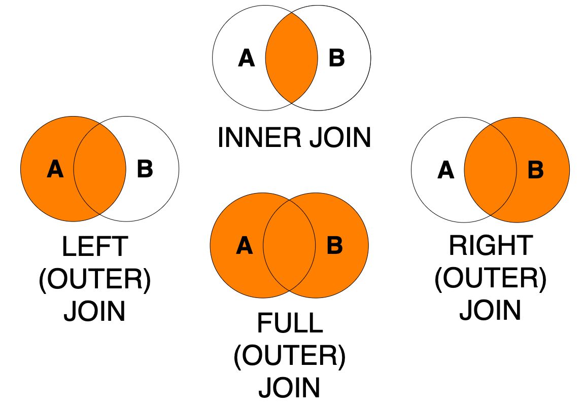
As discussed in the lecture, the dplyr library offers different types of join operations, which correspond to the different SQL joins illustrated in the image below. The use and implications of these different types of joins will be discussed in more detail in the GY7708 module next semester.
Please take your time to understand the example below and check out the related dplyr help pages before continuing. The first four examples execute the exact same full join operation using three different syntaxes: with or without using the pipe operator, and specifying the by argument or not. Note that all those approaches to writing the join are valid and produce the same result. The choice about which approach to use will depend on the code you are writing. In particular, you might find it useful to use the syntax that uses the pipe operator when the join operation is itself only one stem in a series of data manipulation steps. Using the by argument is usually advisable unless you are certain that you aim to join two tables with all and exactly the column that have the same names in the two table.
Note how the result of the join operations is not saved to a variable. The function kable is added after each join operation through a pipe %>% to display the resulting table in a nice format.
city_telephone_prexix <- data.frame(
    city = c("Leicester", "Birmingham"),
    telephon_prefix = c("0116", "0121")
  ) %>%
  as_tibble()

city_telephone_prexix %>%
kable()| city | telephon_prefix |
|---|---|
| Leicester | 0116 |
| Birmingham | 0121 |
# Option 1: without using the pipe operator

# full join verb
full_join(
    # left table
    city_info_wide,
    # right table
    city_telephone_prexix,
    # columns to match
    by = c("city" = "city")
  ) %>%
kable()| city | population | area | density | telephon_prefix |
|---|---|---|---|---|
| Leicester | 329839 | 73.3 | 4500 | 0116 |
| Nottingham | 321500 | 74.6 | 4412 | NA |
| Birmingham | NA | NA | NA | 0121 |
# Option 2: without using the pipe operator
#   and without using the argument "by"
#   as columns have the same name
#   in the two tables.
# Same result as Option 1

# full join verb
full_join(
    # left table
    city_info_wide,
    # right table
    city_telephone_prexix
  ) %>%
kable()| city | population | area | density | telephon_prefix |
|---|---|---|---|---|
| Leicester | 329839 | 73.3 | 4500 | 0116 |
| Nottingham | 321500 | 74.6 | 4412 | NA |
| Birmingham | NA | NA | NA | 0121 |
# Option 3: using the pipe operator
#   and without using the argument "by"
#   as columns have the same name
#   in the two tables.
# Same result as Option 1 and 2

# left table
city_info_wide %>%
  # full join verb
  full_join(
    # right table
    city_telephone_prexix
  ) %>%
kable()| city | population | area | density | telephon_prefix |
|---|---|---|---|---|
| Leicester | 329839 | 73.3 | 4500 | 0116 |
| Nottingham | 321500 | 74.6 | 4412 | NA |
| Birmingham | NA | NA | NA | 0121 |
# Option 4: using the pipe operator
#   and using the argument "by".
# Same result as Option 1, 2 and 3

# left table
city_info_wide %>%
  # full join verb
  full_join(
    # right table
    city_telephone_prexix,
    # columns to match
    by = c("city" = "city")
  ) %>%
kable()| city | population | area | density | telephon_prefix |
|---|---|---|---|---|
| Leicester | 329839 | 73.3 | 4500 | 0116 |
| Nottingham | 321500 | 74.6 | 4412 | NA |
| Birmingham | NA | NA | NA | 0121 |
# Left join
# Using syntax similar to Option 1 above

# left join
left_join(
    # left table
    city_info_wide,
    # right table
    city_telephone_prexix,
    # columns to match
    by = c("city" = "city")
  ) %>%
kable()| city | population | area | density | telephon_prefix |
|---|---|---|---|---|
| Leicester | 329839 | 73.3 | 4500 | 0116 |
| Nottingham | 321500 | 74.6 | 4412 | NA |
# Right join
# Using syntax similar to Option 2 above

# right join verb
right_join(
    # left table
    city_info_wide,
    # right table
    city_telephone_prexix
  ) %>%
kable()| city | population | area | density | telephon_prefix |
|---|---|---|---|---|
| Leicester | 329839 | 73.3 | 4500 | 0116 |
| Birmingham | NA | NA | NA | 0121 |
# Inner join
# Using syntax similar to Option 3 above

# left table
city_info_wide %>%
  # inner join
  inner_join(
    # right table
    city_telephone_prexix
  ) %>%
kable()| city | population | area | density | telephon_prefix |
|---|---|---|---|---|
| Leicester | 329839 | 73.3 | 4500 | 0116 |
4.3 Data: Indices of Multiple Deprivation
Open the Leicester_population project created for the previous chapter. Create a new RMarkdown document using “Exploring deprivation indices in Leicester” as the title and PDF as the output file type. Delete the example code after the setup chunk. Add a new markdown second-heading section named Libraries and a chunk loading the tidyverse and knitr libraries (see below). Save the file with the name exploring_Leicester_deprivation.Rmd in the Leicester_population project.
Download from Blackboard (or the data folder of the repository) the file IndexesMultipleDeprivation2015_Leicester.csv and upload the file to the Leicester_population folder by clicking on the Upload button and selecting the files from your computer.
The Indices of Multiple Deprivation 2015 (see map at cdrc.ac.uk) are based on a series of variables across seven distinct domains of deprivation which are combined to calculate the Index of Multiple Deprivation 2015 (IMD 2015). That is an overall measure of multiple deprivations experienced by people living in an area. These indexes are calculated for every Lower layer Super Output Area (LSOA), which are larger geographic units than the OAs used for the 2011 OAC. The dataset in the file IndexesMultipleDeprivation2015_Leicester.csv contains the main Index of Multiple Deprivation, as well as the values for the seven distinct domains of deprivation and two additional indexes regarding deprivation affecting children and older people. The dataset includes scores, ranks (where 1 indicates the most deprived area), and decile (i.e., the first decile includes the 10% most deprived areas in England).
The code below loads the IMD 2015 dataset.
# Load Indexes of Multiple deprivation data
leicester_IMD2015 <-
  read_csv("IndexesMultipleDeprivation2015_Leicester.csv")
leicester_2011OAC <-
  read_csv("2011_OAC_Raw_uVariables_Leicester.csv")
4.4 Working with multiple tables
4.4.1 From long to wide table
The IMD 2015 data are in a long format, which means that every area is represented by more than one row: the column Value presents the value; the column IndicesOfDeprivation indicates which index the value refers to; the column Measurement indicates whether the value is a score, rank, or decile. The code below illustrates the data format used for the IndicesOfDeprivation table, and showing the rows for the LSOA including the University of Leicester (feature code E01013649).
leicester_IMD2015 %>%
  filter(FeatureCode == "E01013649") %>%
  select(FeatureCode, IndicesOfDeprivation, Measurement, Value) %>%
kable()| FeatureCode | IndicesOfDeprivation | Measurement | Value |
|---|---|---|---|
| E01013649 | Income Deprivation Domain | Score | 0.070 |
| E01013649 | Employment Deprivation Domain | Score | 0.075 |
| E01013649 | Income Deprivation Affecting Children Index (IDACI) | Score | 0.087 |
| E01013649 | Income Deprivation Affecting Older People Index (IDAOPI) | Score | 0.153 |
| E01013649 | Health Deprivation and Disability Domain | Score | 0.272 |
| E01013649 | Index of Multiple Deprivation (IMD) | Score | 19.665 |
| E01013649 | Education, Skills and Training Domain | Score | 2.195 |
| E01013649 | Barriers to Housing and Services Domain | Score | 14.324 |
| E01013649 | Living Environment Deprivation Domain | Score | 57.197 |
| E01013649 | Crime Domain | Score | 1.159 |
| E01013649 | Income Deprivation Domain | Rank | 23511.000 |
| E01013649 | Index of Multiple Deprivation (IMD) | Rank | 14539.000 |
| E01013649 | Employment Deprivation Domain | Rank | 21227.000 |
| E01013649 | Education, Skills and Training Domain | Rank | 30744.000 |
| E01013649 | Barriers to Housing and Services Domain | Rank | 23885.000 |
| E01013649 | Health Deprivation and Disability Domain | Rank | 12269.000 |
| E01013649 | Living Environment Deprivation Domain | Rank | 1197.000 |
| E01013649 | Crime Domain | Rank | 2214.000 |
| E01013649 | Income Deprivation Affecting Children Index (IDACI) | Rank | 22984.000 |
| E01013649 | Income Deprivation Affecting Older People Index (IDAOPI) | Rank | 16055.000 |
| E01013649 | Employment Deprivation Domain | Decile | 7.000 |
| E01013649 | Income Deprivation Affecting Older People Index (IDAOPI) | Decile | 5.000 |
| E01013649 | Barriers to Housing and Services Domain | Decile | 8.000 |
| E01013649 | Income Deprivation Affecting Children Index (IDACI) | Decile | 7.000 |
| E01013649 | Crime Domain | Decile | 1.000 |
| E01013649 | Income Deprivation Domain | Decile | 8.000 |
| E01013649 | Health Deprivation and Disability Domain | Decile | 4.000 |
| E01013649 | Living Environment Deprivation Domain | Decile | 1.000 |
| E01013649 | Education, Skills and Training Domain | Decile | 10.000 |
| E01013649 | Index of Multiple Deprivation (IMD) | Decile | 5.000 |
In the following section, the analysis aims to explore how certain census variables vary in areas with different deprivation levels. Thus, we need to extract the Decile rows from the IMD 2015 dataset and transform the data in a wide format, where each index is represented as a separate column.
To that purpose, we also need to change the name of the indexes slightly, to exclude spaces and punctuation, so that the new column names are simpler than the original text, and can be used as column names. That part of the manipulation is performed using mutate and functions from the stringr library.
leicester_IMD2015_decile_wide <- leicester_IMD2015 %>%
  # Select only Socres
  filter(Measurement == "Decile") %>%
  # Trim names of IndicesOfDeprivation
  mutate(
    IndicesOfDeprivation = str_replace_all(IndicesOfDeprivation, "\\s", "")
  ) %>%
  mutate(
    IndicesOfDeprivation = str_replace_all(IndicesOfDeprivation, "[:punct:]", "")
  ) %>%
  mutate(
    IndicesOfDeprivation = str_replace_all(IndicesOfDeprivation, "\\(", "")
  ) %>%
  mutate(
    IndicesOfDeprivation = str_replace_all(IndicesOfDeprivation, "\\)", "")
  ) %>%
  # Spread
  pivot_wider(
    names_from = IndicesOfDeprivation,
    values_from = Value
  ) %>%
  # Drop columns
  select(-DateCode, -Measurement, -Units)
Let’s compare the columns of the original long IMD 2015 dataset with the wide dataset created above, using the function colnames.
## [1] "FeatureCode"          "DateCode"
## [3] "Measurement"          "Units"
## [5] "Value" "IndicesOfDeprivation"## [1] "FeatureCode"
## [2] "HealthDeprivationandDisabilityDomain"
## [3] "IncomeDeprivationAffectingOlderPeopleIndexIDAOPI"
## [4] "BarrierstoHousingandServicesDomain"
## [5] "EmploymentDeprivationDomain"
## [6] "EducationSkillsandTrainingDomain"
## [7] "LivingEnvironmentDeprivationDomain"
## [8] "IncomeDeprivationAffectingChildrenIndexIDACI"
## [9] "CrimeDomain"
## [10] "IndexofMultipleDeprivationIMD"
## [11] "IncomeDeprivationDomain"In leicester_IMD2015_decile_wide, we now have only one row representing the LSOA including the University of Leicester (feature code E01013649) and the main Index of Multiple Deprivations is now represented by the column IndexofMultipleDeprivationIMD. The value reported is the same – that is 5, which means that the selected LSOA is estimated to be in the range 40-50% most deprived areas in England – but we changed the data format.
# Original long IMD 2015 dataset
leicester_IMD2015 %>%
  filter(
    FeatureCode == "E01013649",
    IndicesOfDeprivation == "Index of Multiple Deprivation (IMD)",
    Measurement == "Decile"
  ) %>%
  select(FeatureCode, IndicesOfDeprivation, Measurement, Value) %>%
kable()| FeatureCode | IndicesOfDeprivation | Measurement | Value |
|---|---|---|---|
| E01013649 | Index of Multiple Deprivation (IMD) | Decile | 5 |
# New wide IMD 2015 dataset
leicester_IMD2015_decile_wide %>%
  filter(FeatureCode == "E01013649") %>%
  select(FeatureCode, IndexofMultipleDeprivationIMD) %>%
kable()| FeatureCode | IndexofMultipleDeprivationIMD |
|---|---|
| E01013649 | 5 |
4.4.2 Joining tables
As discussed above, two tables can be joined using a common column of identifiers. We can thus join the 2011 OAC and the IMD 2015 datasets into a single table. The LSOA code included in the 2011 OAC table is used to match that information with the corresponding row in the IMD 2015. The resulting table provides all the information from the 2011 OAC for each OA, plus the Index of Multiple Deprivations decile for the LSOA containing each OA.
That operation can be carried out using the function inner_join, and specifying the common column (or columns, if more than one is to be used as identifier) as argument of by. Note that using inner_join would result in dropping any row which doesn’t have a match in the other table, either way. In this case, that should not happen, as all OAs are part of an LSOA, and any LSOA contains at least one OA.
leicester_2011OAC_IMD2015 <-
  leicester_2011OAC %>%
  inner_join(
    leicester_IMD2015_decile_wide,
    by = c("LSOA11CD" = "FeatureCode")
  )
As each LSOA contains multiple OAs, each row from the leicester_IMD2015_decile_wide table is matched to multiple rows from the leicester_2011OAC table. For instance, as shown in the table below, the information from the IMD 2015 dataset about the LSOA encompassing the University of Leicester (feature code E01013649) is joined to multiple rows from the 2011 OAC dataset, including the OA encompassing the University of Leicester (feature code E00068890) as well as other neighbouring OAs.
leicester_2011OAC_IMD2015 %>%
  # Note that the LSOA11CD column needs to be used
  # as the previous join as combined
  # LSOA11CD and FeatureCode
  # into one, name LSOA11CD
  filter(LSOA11CD == "E01013649") %>%
  select(OA11CD, LSOA11CD, supgrpname, IndexofMultipleDeprivationIMD) %>%
kable()| OA11CD | LSOA11CD | supgrpname | IndexofMultipleDeprivationIMD |
|---|---|---|---|
| E00169447 | E01013649 | Cosmopolitans | 5 |
| E00168083 | E01013649 | Cosmopolitans | 5 |
| E00068893 | E01013649 | Cosmopolitans | 5 |
| E00068892 | E01013649 | Cosmopolitans | 5 |
| E00068890 | E01013649 | Cosmopolitans | 5 |
Once the result is stored into the variable leicester_2011OAC_IMD2015, further analysis can be carried out. For instance, count can be used to count how many OAs fall into each 2011 OAC supergroup and decile of the Index of Multiple Deprivations.
| supgrpname | IndexofMultipleDeprivationIMD | n |
|---|---|---|
| Constrained City Dwellers | 1 | 30 |
| Constrained City Dwellers | 2 | 3 |
| Constrained City Dwellers | 3 | 2 |
| Constrained City Dwellers | 6 | 1 |
| Cosmopolitans | 2 | 25 |
| Cosmopolitans | 3 | 15 |
| Cosmopolitans | 4 | 15 |
| Cosmopolitans | 5 | 8 |
| Cosmopolitans | 6 | 10 |
| Cosmopolitans | 8 | 10 |
| Ethnicity Central | 1 | 28 |
| Ethnicity Central | 2 | 18 |
| Ethnicity Central | 3 | 5 |
| Ethnicity Central | 4 | 5 |
| Ethnicity Central | 5 | 1 |
| Hard-Pressed Living | 1 | 68 |
| Hard-Pressed Living | 2 | 24 |
| Hard-Pressed Living | 3 | 5 |
| Hard-Pressed Living | 5 | 3 |
| Hard-Pressed Living | 6 | 1 |
| Multicultural Metropolitans | 1 | 107 |
| Multicultural Metropolitans | 2 | 119 |
| Multicultural Metropolitans | 3 | 132 |
| Multicultural Metropolitans | 4 | 100 |
| Multicultural Metropolitans | 5 | 56 |
| Multicultural Metropolitans | 6 | 34 |
| Multicultural Metropolitans | 7 | 6 |
| Multicultural Metropolitans | 8 | 17 |
| Multicultural Metropolitans | 9 | 2 |
| Suburbanites | 2 | 2 |
| Suburbanites | 3 | 2 |
| Suburbanites | 4 | 2 |
| Suburbanites | 5 | 10 |
| Suburbanites | 6 | 11 |
| Suburbanites | 7 | 16 |
| Suburbanites | 8 | 3 |
| Suburbanites | 9 | 8 |
| Urbanites | 1 | 1 |
| Urbanites | 2 | 3 |
| Urbanites | 3 | 5 |
| Urbanites | 4 | 15 |
| Urbanites | 5 | 14 |
| Urbanites | 6 | 4 |
| Urbanites | 7 | 12 |
| Urbanites | 8 | 7 |
| Urbanites | 9 | 4 |
As another example, the code below can be used to group OAs based on the decile and then calculate the percentage of adults not in employment using the u074 (No adults in employment in household: With dependent children) and u075 (No adults in employment in household: No dependent children) variables from the 2011 OAC dataset.
leicester_2011OAC_IMD2015 %>%
  group_by(IndexofMultipleDeprivationIMD) %>%
  summarise(
    adults_not_empl_perc = (sum(u074 + u075) / sum(Total_Population)) * 100
  ) %>%
kable()| IndexofMultipleDeprivationIMD | adults_not_empl_perc |
|---|---|
| 1 | 17.071876 |
| 2 | 14.191205 |
| 3 | 10.405029 |
| 4 | 9.966309 |
| 5 | 11.337036 |
| 6 | 10.710509 |
| 7 | 10.641026 |
| 8 | 9.686658 |
| 9 | 9.898140 |
4.5 Exercise 104.1
Extend the “Exploring deprivation indices in Leicester” document to include the code necessary to solve the questions below. Use the full list of variable names from the 2011 UK Census used to generate the 2011 OAC that can be found in the file 2011_OAC_Raw_uVariables_Lookup.csv to indetify which columns to use to complete the tasks.
Question 104.1.1: Write a piece of code using the pipe operator and the dplyr library to generate a table showing the percentage of EU citizens over total population, calculated grouping OAs by the related decile of the Index of Multiple Deprivations, but only accounting for areas classified as Cosmopolitans or Ethnicity Central or Multicultural Metropolitans.
Question 104.1.2: Write a piece of code using the pipe operator and the dplyr library to generate a table showing the percentage of EU citizens over total population, calculated grouping OAs by the related supergroup in the 2011 OAC, but only accounting for areas in the top 5 deciles of the Index of Multiple Deprivations.
Question 104.1.3: Write a piece of code using the pipe operator and the dplyr library to generate a table showing the percentage of people aged 65 and above, calculated grouping OAs by the related supergroup in the 2011 OAC and decile of the Index of Multiple Deprivations, and ordering the table by the calculated value in a descending order.
Question 104.1.4: Write a piece of code using the pipe operator and the dplyr and tidyr libraries to generate a long format of the leicester_2011OAC_IMD2015 table only including the values (census variables) used in Question 104.1.3.
Question 104.1.5: Write a piece of code using the pipe operator and the dplyr and tidyr libraries to generate a table similar to the one generated for Question 104.1.4, but showing the values as percentages over total population.
by Stef De Sabbata – text licensed under the CC BY-SA 4.0, contains public sector information licensed under the Open Government Licence v3.0, code licensed under the GNU GPL v3.0.